Evolution of Multiple Object Detection and the Rise of YOLO

Evolution of Multiple Object Detection and the Rise of YOLO

Object detection is the action of detecting what objects are in an image, and pinpointng where each object is located. This task lies at the core of many real-world applications such as autonomous driving, medical imaging, video surveillance, and more.

Early methods such as Deformable Part Models (DPM) relied on sliding windows, while R-CNN introduced Convolutional Neural Networks (CNNs) for feature extraction to improve accuracy. These approaches, however, were too slow for real-time use.

The breakthrough came with YOLO (You Only Look Once) in 2016, which reframed detection as a single regression problem. This shift made object detection both fast and accurate, enabling real-time applications. In this post, I’ll look at the background of object detection, how YOLO works, its architecture, and its loss function.

What is Multiple Object Detection?

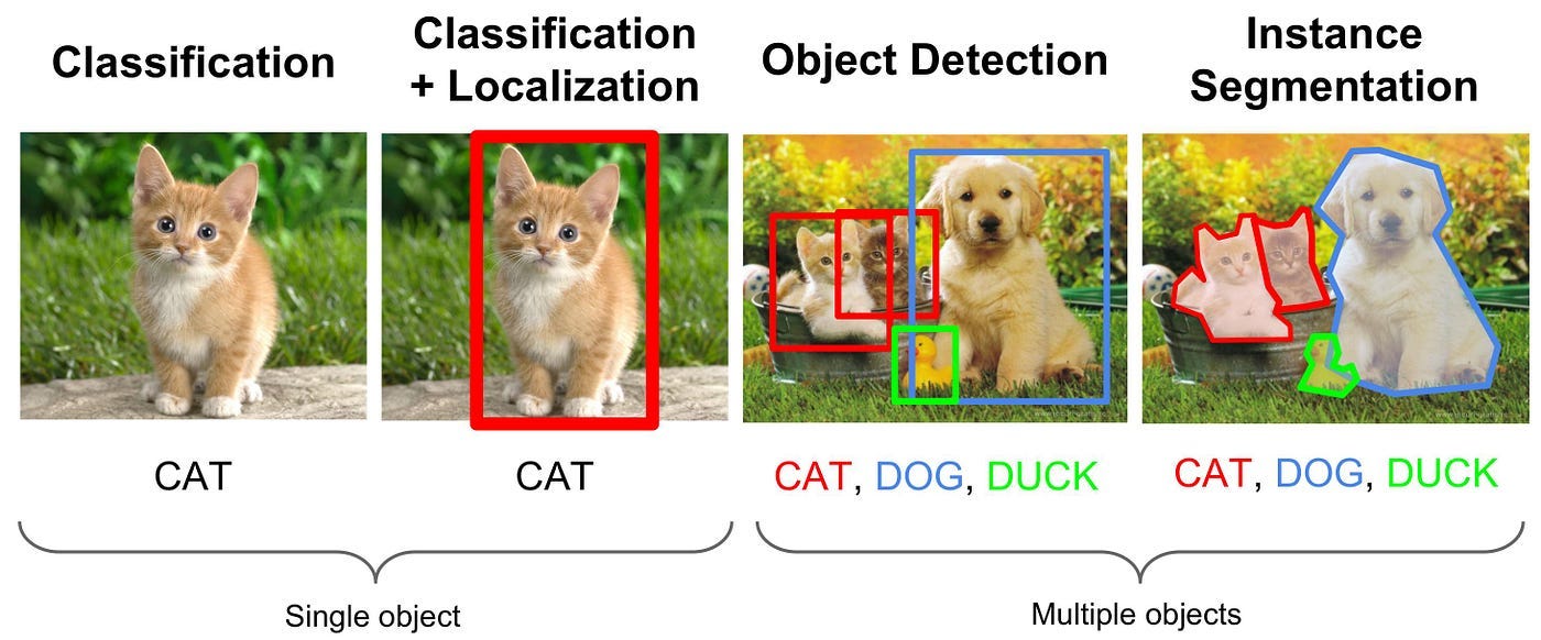
Multiple object detection is the task of identifying all objects in an image by determining both what they are (classification) and where they are located (localization).

• Classification: Identifies what object (only one) is in the image (e.g., “CAT”).
• Classification + Localization: Identifies what’s in the image and where it is (bounding box).
• Multiple Object Detection: Detects multiple objects in the same scene, with bounding boxes for all of them.
• Instance Segmentation: Extends detection by outlining the exact shapes of the objects instead of simple bounding boxes.

Before YOLO

Deformable Parts Model

---

The Deformable Parts Model (DPM) was a pioneering object detection method that predated deep-learning approaches like R-CNN. It was introduced by Pedro Felzenszwalb et al. in 2008, and quickly became the state-of-the-art (SOTA) approach in object detection for several years.

---

How It Works

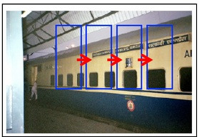
1. Sliding Window
   The model slides a bounding box (window) across the image at regular pixel intervals to examine different regions.

1. Block-wise Operation
   Each region is divided into small fixed-size blocks (e.g., 8×8 pixels). These blocks form the basis for feature extraction.

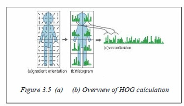
1. HOG Feature Extraction
   For each block within a bounding box, histogram of oriented gradients (HOG) features (or similar such as SIFT) are computed. These features capture local texture and shape.

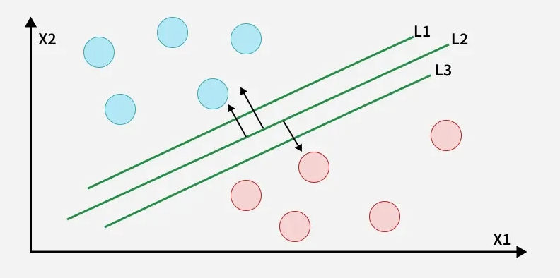
2. Template Matching / Classification
   Templates (or filters) pre-trained for specific object parts—such as a root filter for an entire object and part filters for subregions—are matched against the HOG features of the corresponding blocks. Each filter’s alignment produces a score (often using an SVM classifier), and the sum of these scores determines whether the object is detected.

1. Feature Ensemble
   The final detection decision aggregates scores from multiple templates, effectively forming an ensemble of classifiers that confirm the presence of an object in that window.

R-CNNs

---

Now, did DPM remind you of something? Windows with certain sizes sliding through an image, caculating feature values along the way..

Yes exactly! CNNs!

*That was one of my favorite aha moments while studying object detection

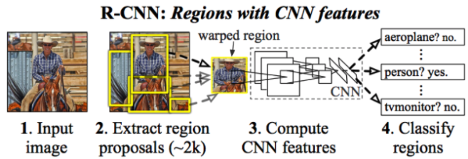
It was just a matter of time untill somebody came up with the idea to use CNNs for object detection, especially after AlexNet in 2012. Evidently, Ross Girshick et al. introduced R-CNN in 2014. Using CNN for feature vector extraction, which were to fed into SVMs for classification.

---

How It Works

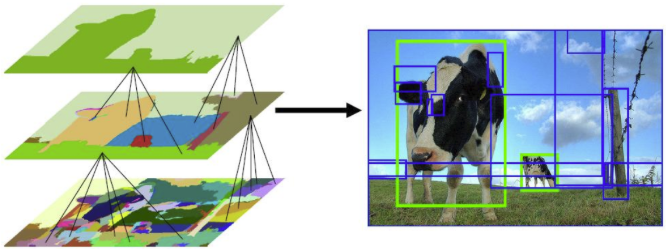
1. Region Proposals
   Instead of scanning the entire image with sliding windows, R-CNN first generated around 2,000 region proposals (candidate object locations) using algorithms like Selective Search.

2. Feature Extraction with CNNs
   Each region proposal was cropped and passed through a pre-trained CNN (e.g., AlexNet) to extract features.

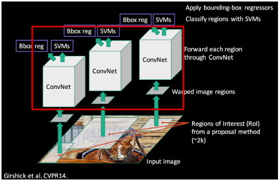
1. Classification and Refinement
   • A separate SVM classifier determined the object category for each region.
   • A bounding-box regressor adjusted and refined the coordinates for higher accuracy.

You Only Look Once: Unified, Real-Time Object Detection

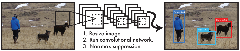
YOLO, short for You Only Look Once, introduced a revolutionary idea: instead of treating detection as a multi-stage process, YOLO reframes object detection as a single regression problem.

• Input: raw image pixels (D x H x W)
• Output: bounding box coordinates + class probabilities (S x S x (C + B*5))

This means YOLO looks at the image just once (hence the name), and directly predicts what objects are present and where they are. This design eliminates the need for region proposals and repeated classification, making YOLO exceptionally fast and suitable for real-time detection.

YOLO’s Architecture

---

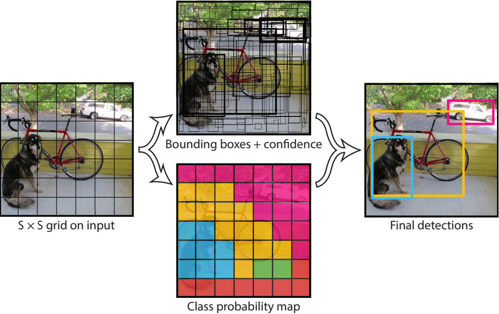
• The image is divided into an S × S grid. Each grid cell predicts:
  • B bounding box coordinates (x, y, width, height)
  • A confidence score
  • C class probabilities
• Hence, the model outputs a tensor with shape of [BATCH SIZE, C + B*5, S, S]
  • For the PASCAL VOC, C = 20
  • and the paper states that each gird only produces 2 bound boxes, so B = 2
  • and S = 7
• For me personally, I’d like to interpret it backwards. Instead of thinking about splitting the input image into S x S grid, I focused more on how the ouput is S x S, and how each grid would need to have a big enough receptive field on the input image.
• That makes much more sense since each grid in the output should be able to see the whole image, or at least its close neighbouring grids in the input image, for the model to truly figure out the center of the object along with the width and the height of the bounding boxes.
• The concept of assuring a big enough receptive field on the input image for the ouput, really plays an important role here.

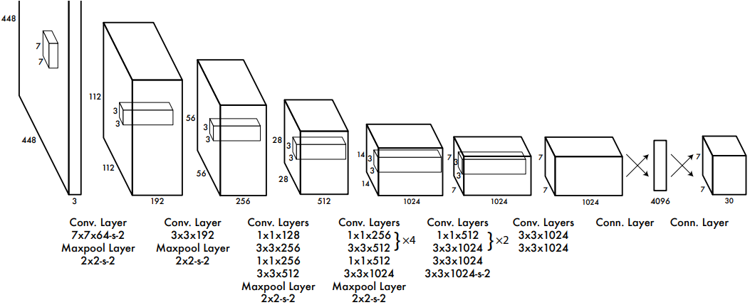
• Then the network consists of 24 convolutional layers (called darknet) followed by 2 fully connected layers.
• For activations, it uses Leaky ReLU for most layers, while the final layer uses a linear activation to output bounding box coordinates.

By combining these, YOLO produces dense predictions for the entire image in a single forward pass.

YOLO’s Loss Function

---

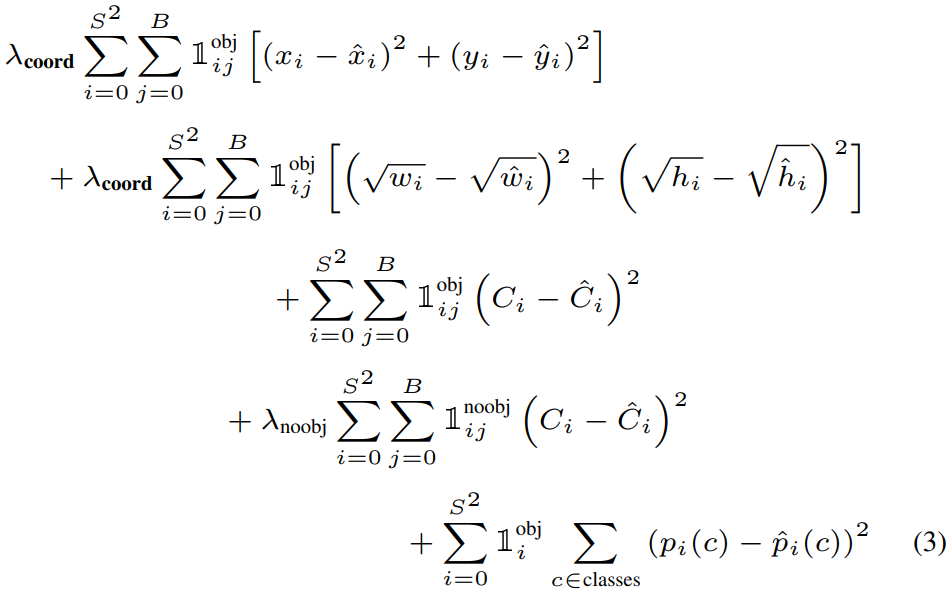
YOLO’s loss function is a sum of multiple components that balance localization accuracy, confidence, and classification. The overall goal is to penalize wrong bounding boxes, wrong objectness scores, and wrong class predictions.

1. Localization Loss (Bounding Box Coordinates)

\[\lambda_{coord} \sum_{i=0}^{S^2} \sum_{j=0}^{B} 1_{ij}^{obj} \left[(x_i - \hat{x}_i)^2 + (y_i - \hat{y}_i)^2\right]\]

• Penalizes error in the center coordinates (x, y) of the bounding box.
• Only applied if the predictor is responsible for an object ($1_{ij}^{obj}=1$).
• Weighted by λ_coord (usually 5) to emphasize precise localization.

2. Localization Loss (Bounding Box Size)

\[\lambda_{coord} \sum_{i=0}^{S^2} \sum_{j=0}^{B} 1_{ij}^{obj} \left[(\sqrt{w_i} - \sqrt{\hat{w}_i})^2 + (\sqrt{h_i} - \sqrt{\hat{h}_i})^2\right]\]

• Penalizes error in the width (w) and height (h) of the bounding box.
• Uses square roots of w and h instead of raw values to reduce sensitivity to large boxes (so small object errors are weighted more fairly).
• Also weighted by λ_coord (≈5).

3. Confidence Loss (Object Present)

\[\sum_{i=0}^{S^2} \sum_{j=0}^{B} 1_{ij}^{obj} (C_i - \hat{C}_i)^2\]

• Confidence score $C_i$ represents IoU (Intersection over Union) between predicted and ground-truth box + probability of an object being present.
• This term penalizes error when an object is present.

4. Confidence Loss (No Object Present)

\[\lambda_{noobj} \sum_{i=0}^{S^2} \sum_{j=0}^{B} 1_{ij}^{noobj} (C_i - \hat{C}_i)^2\]

• When no object is present in a cell ($1_{ij}^{noobj}=1$), the confidence score should ideally be 0.
• Penalizes false positives (predicting high confidence when there’s no object).
• Weighted by λ_noobj (≈0.5) to avoid overwhelming the loss, since most grid cells have no objects.

5. Classification Loss

\[\sum_{i=0}^{S^2} 1_i^{obj} \sum_{c \in classes} (p_i(c) - \hat{p}_i(c))^2\]

• Applied only to cells containing an object.
• Penalizes error between predicted class probabilities $p_i(c)$ and true labels $\hat{p}_i(c)$.
• Uses sum-squared error for all classes.

---

The Role of λ (Lambdas)

• λ_coord (5): Increases weight of localization error (bounding box coordinates + size). Without this, classification and confidence terms would dominate.
• λ_noobj (0.5): Decreases weight for background confidence error, since most cells have no objects and would otherwise overwhelm the loss.

Advance in Research?

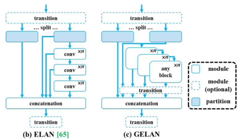
• YOLO v9 – Learning What You Want to Learn Using Programmable Gradient Information (2024)
  Introduces Programmable Gradient Information (PGI) to improve training signals and the Generalized Efficient Layer Aggregation Network (GELAN) (a generalization of ELAN) for efficient architecture design.

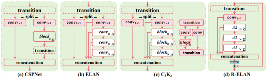
• YOLO v12 – Attention-Centric Object Detection (2025)
  Proposes an attention-centric YOLO that keeps real-time speed. Key components are the Area Attention module (A2) and Residual Efficient Layer Aggregation Networks (R-ELAN)

Implementing with PyTorch

The architecture is basically in the paper, and so is the loss. It is relatively straightforward and easy to code. So you can check it out in my GitHub repo.

• https://github.com/kmsrogerkim/AI-Models-Collection

And I would have to give credit to Aladdin Persson for implementing the model and everything else prior to me.

• https://github.com/aladdinpersson/Machine-Learning-Collection/tree/master/ML/Pytorch/object_detection/YOLO

References

• Redmon, J., Divvala, S., Girshick, R., & Farhadi, A. (2016). You only look once: Unified, real-time object detection. In Proceedings of the IEEE Conference on Computer Vision and Pattern Recognition (CVPR) (pp. 779–788).

• Wang, C.-Y., Yeh, I.-H., & Liao, H.-Y. M. (2024). YOLOv9: Learning what you want to learn using programmable gradient information. In European Conference on Computer Vision (ECCV). Cham: Springer Nature Switzerland.

• Tian, Y., Ye, Q., & Doermann, D. (2025). YOLOv12: Attention-centric real-time object detectors. arXiv preprint arXiv:2502.12524.

• Augmented Startups. (2023). Object detection vs classification in computer vision. Medium. Retrieved from https://augmentedstartups.medium.com/object-detection-vs-classification-in-computer-vision-123c437e33be

• 89douner. (2020). [Deformable Parts Model Explanation]. Tistory Blog. Retrieved from https://89douner.tistory.com/82

• Ganghee Lee. (2020). [R-CNN Object Detection Explanation]. Tistory Blog. Retrieved from https://ganghee-lee.tistory.com/35

  Written by

  Roger Kim