<?xml version="1.0" encoding="utf-8"?><feed xmlns="http://www.w3.org/2005/Atom" ><generator uri="https://jekyllrb.com/" version="3.10.0">Jekyll</generator><link href="https://kmsrogerkim.github.io/feed.xml" rel="self" type="application/atom+xml" /><link href="https://kmsrogerkim.github.io/" rel="alternate" type="text/html" /><updated>2026-05-28T16:58:08+00:00</updated><id>https://kmsrogerkim.github.io/feed.xml</id><title type="html">Roger’s Blog</title><subtitle>This is where I share my journey to becoming a backend developer!</subtitle><author><name>Roger Kim</name></author><entry><title type="html">8 Essential Computer Vision Papers I Read as a CS Undergrad: From VAE to DiT</title><link href="https://kmsrogerkim.github.io/ai/essential-cv-papers/" rel="alternate" type="text/html" title="8 Essential Computer Vision Papers I Read as a CS Undergrad: From VAE to DiT" /><published>2026-02-23T00:00:00+00:00</published><updated>2026-02-23T00:00:00+00:00</updated><id>https://kmsrogerkim.github.io/ai/essential-cv-papers</id><content type="html" xml:base="https://kmsrogerkim.github.io/ai/essential-cv-papers/"><![CDATA[<p>Here are 8 essential computer vision papers I read that forms the foundation of modern computer vision / generative models; in chronological order.</p>

<ol>
  <li><a href="https://arxiv.org/abs/1312.6114">Variational Autoencoder (VAE) (2013)</a></li>
  <li><a href="https://arxiv.org/abs/2006.11239">Denoising Diffusion Probabilistic Models (DDPM) (2020)</a></li>
  <li><a href="https://arxiv.org/abs/2010.11929">Vision Transformer (ViT) (2020)</a></li>
  <li><a href="https://arxiv.org/abs/2103.00020">Contrastive Language-Image Pretraining (CLIP) (2021)</a></li>
  <li><a href="https://arxiv.org/abs/2207.12598">Classifier-Free Guidance (CFG) (2021)</a></li>
  <li><a href="https://arxiv.org/abs/2111.06377">Masked Autoencoder (MAE) (2021)</a></li>
  <li><a href="https://arxiv.org/abs/2112.10752">Latent Diffusion Models (LDM) (2022)</a></li>
  <li><a href="https://arxiv.org/abs/2212.09748">Diffusion Transformer (DiT) (2022)</a></li>
</ol>

<p>Modern computer vision and generative modeling evolved through a sequence of connected breakthroughs. In 2013, the Variational Autoencoder (VAE) introduced probabilistic latent-variable modeling and the Evidence Lower Bound (ELBO), providing a practical framework for learning continuous latent representations. Instead of mapping an image into a fixed deterministic vector, VAE modeled the latent space as a distribution, which later became important for scalable generative models and latent-space compression.</p>

<p>For several years, generative models struggled with either unstable training, low sample quality, or limited diversity. In 2020, Denoising Diffusion Probabilistic Models (DDPM) changed the direction of the field by framing image generation as iterative denoising. Rather than generating an image in a single step, DDPM learned to reverse a Markov noising process and gradually recover data from Gaussian noise. Diffusion models produced significantly higher visual fidelity and more stable training behavior than many previous approaches, quickly becoming one of the dominant paradigms in image synthesis. However, diffusion models were computationally expensive because the generation process required many sequential denoising steps and operated directly in high-dimensional pixel space.</p>

<p>During the same period, Vision Transformer (ViT) introduced transformers into computer vision by treating image patches as token sequences. This reduced dependence on convolutional inductive bias and showed that transformer scaling behavior could extend beyond natural language processing. In 2021, Masked Autoencoders (MAE) further strengthened transformer-based vision learning through self-supervised masked reconstruction, allowing ViTs to learn efficient image representations from large-scale unlabeled data. Together, ViT and MAE established transformers as scalable backbone architectures for future generative vision systems.</p>

<p>Also in 2021, CLIP replaced closed-set classification objectives with contrastive image-text representation learning. Instead of predicting fixed labels, CLIP learned a shared embedding space between images and natural language, which later became critical for prompt-conditioned image generation systems. In the same year, Classifier-Free Guidance (CFG) solved another major limitation of diffusion models: weak conditional control. By combining conditional and unconditional diffusion predictions during sampling, CFG greatly improved prompt alignment without requiring an external classifier, making controllable text-to-image generation practical.</p>

<p>In 2022, Latent Diffusion Models (LDM) combined many of these developments into a single efficient framework. LDM used VAE-based latent compression to avoid diffusion in pixel space, reducing computational cost while preserving image quality. It used DDPM-style denoising as the generative mechanism and relied on CLIP-based text conditioning together with CFG-based sampling guidance for controllable generation. LDM demonstrated that high-resolution text-to-image synthesis could become both practical and scalable, and it became the foundation of systems such as Stable Diffusion.</p>

<p>Later in 2022, Diffusion Transformers (DiT) replaced the U-Net diffusion backbone with transformer architectures derived from the ViT lineage. DiT showed that transformers were not only effective for representation learning, but also highly scalable for diffusion-based image generation itself. This marked a broader transition toward transformer-native generative vision systems and influenced later work in image, video, and multimodal generation.</p>

<p>This blog post goes through the core ideas, mathematical formulations, and architectural contributions introduced by each paper, with a focus on how these works connect to each other historically and technically. Rather than treating these papers as isolated breakthroughs, the goal is to examine how concepts such as latent-variable modeling, diffusion-based generation, transformer architectures, self-supervised learning, and multimodal conditioning gradually built the foundation of modern computer vision and generative AI systems. Through this progression, the post introduces eight papers that significantly influenced my understanding of the field.</p>

<h2 id="1-variational-autoencoder-vae">1. Variational Autoencoder (VAE)</h2>

<p>A VAE learns an encoder that maps data into a latent distribution and a decoder that reconstructs samples from latent variables. Instead of learning a deterministic representation, VAE approximates the intractable posterior</p>

\[q_\phi(z|x)\approx p_\theta(z|x)\]

<p>where the true posterior and the margianl likelihood are generally expensive to compute exactly.</p>

\[p_\theta(z|x) = \frac{p_\theta(x|z)p(z)}{p_\theta(x)}
\qquad
p_\theta(x) = \int p_\theta(x|z)p(z)dz\]

<p>VAE therefore introduces variational inference and optimizes the Evidence Lower Bound (ELBO) from the original paper:</p>

\[\mathcal{L}(\theta,\phi;x^{(i)})
= 
- D_{KL}\left(q_\phi(z|x^{(i)})||p_\theta(z)\right)
+
\frac{1}{L}\sum_{l=1}^{L}\log p_\theta\left(x^{(i)}|z^{(i,l)}\right)\]

\[z^{(i,l)}

g_\phi\left(\epsilon^{(i,l)},x^{(i)}\right),
\qquad
\epsilon^{(i,l)}\sim p(\epsilon)\]

<p>This formulation introduces the following reparameterization trick which allows gradients to propagate through stochastic latent sampling during backpropagation.</p>

\[z
=
\mu
+
\sigma\odot\epsilon,
\qquad
\epsilon\sim\mathcal{N}(0,I)\]

<h3 id="core-contribution">Core contribution</h3>

<p>VAE introduced:</p>
<ul>
  <li>variational inference for deep generative models</li>
  <li>continuous latent-variable modeling</li>
  <li>the reparameterization trick for differentiable sampling</li>
</ul>

<p>It established the idea that generation can happen inside a structured latent space rather than directly in pixel space. I cannot stretch enough the importance of this paper. It is really, <strong>REALLY</strong> important that you understnad the <strong>ELBO</strong> introduced in this paper. If you would like to dig deeper, please try out this series of blog posts by Professor Yoo.</p>

<ol>
  <li><a href="https://jaejunyoo.blogspot.com/2017/04/auto-encoding-variational-bayes-vae-1.html?m=1">초짜 대학원생의 입장에서 이해하는 Auto-Encoding Variational Bayes (VAE) (1)</a></li>
  <li><a href="https://jaejunyoo.blogspot.com/2017/04/auto-encoding-variational-bayes-vae-2.html?m=1">초짜 대학원생의 입장에서 이해하는 Auto-Encoding Variational Bayes (VAE) (2)</a></li>
</ol>

<p><em>They are written in Korean… but this is the best blog post I could find discussing VAE in such depth and detail.</em></p>

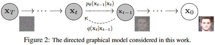
<h2 id="2-denoising-diffusion-probabilistic-models-ddpm">2. Denoising Diffusion Probabilistic Models (DDPM)</h2>

<p align="center">
  <img src="/assets/img/ddpm.png" width="100%" />
</p>

<p>DDPM formulates image generation as iterative denoising. The forward process gradually corrupts data with Gaussian noise:</p>

\[q(x_t|x_{t-1}) =
\mathcal{N}
(
x_t;
\sqrt{1-\beta_t}x_{t-1},
\beta_t I
)\]

<p>After many timesteps $ x_T \sim \mathcal{N}(0, I) $. The model then learns the reverse process which progressively removes noise and reconstructs the data distribution. Mathematically, DDPM remains closely connected to VAE: both introduce latent variables, define tractable Gaussian transitions, and optimize variational lower bounds instead of directly maximizing the intractable data likelihood. DDPM derives a variational objective over the entire diffusion trajectory:</p>

\[\mathcal{L}(\theta,\phi;x^{(i)})
= 
- D_{KL}\left(q_\phi(z|x^{(i)})||p_\theta(z)\right)
+
\frac{1}{L}\sum_{l=1}^{L}\log p_\theta\left(x^{(i)}|z^{(i,l)}\right)\]

<p>which is later simplified into the practical denoising objective:</p>

\[L_{simple} = \mathbb{E}_{x_0,\epsilon,t} \left[\|\epsilon -\epsilon_\theta(x_t, t)\|^2\right]\]

<p>Instead of directly predicting images, DDPM therefore learns to predict the Gaussian noise added at each timestep.</p>

<p>To dive deeper, please refer to <a href="https://kmsrogerkim.github.io/ai/ddpm/">my blog post about DDPM!</a></p>

<h2 id="3-vision-transformer-vit">3. Vision Transformer (ViT)</h2>

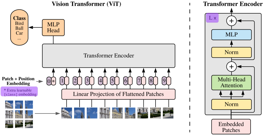
<p>Before ViT, CNNs dominated computer vision because images were assumed to require convolutional inductive biases such as locality and translation equivariance. ViT challenged this assumption by treating images as token sequences.</p>

<p align="center">
  <img src="/assets/img/vit/vit_architecture.png" width="100%" />
</p>

<p>Given an image $x \in \mathbb{R}^{H \times W \times C}$, ViT partitions the image into fixed-size patches:</p>

\[x \rightarrow {x_p^1, x_p^2, ..., x_p^N}\]

<p>Each flattened patch is linearly projected into a token embedding:</p>

\[z_0 = [x_p^1E; x_p^2E; ...; x_p^NE] + E_{pos}\]

<p>The token sequence is then processed through transformer self-attention:</p>

\[\text{softmax}
\left(
\frac{QK^T}{\sqrt d}
\right)V\]

<p>The key result was not merely that transformers work for vision, but that they scale remarkably well with data and model size. ViT fundamentally changed modern vision architectures and later became the foundation for MAE, DiT, and many multimodal generative systems.</p>

<h2 id="4-clip">4. CLIP</h2>

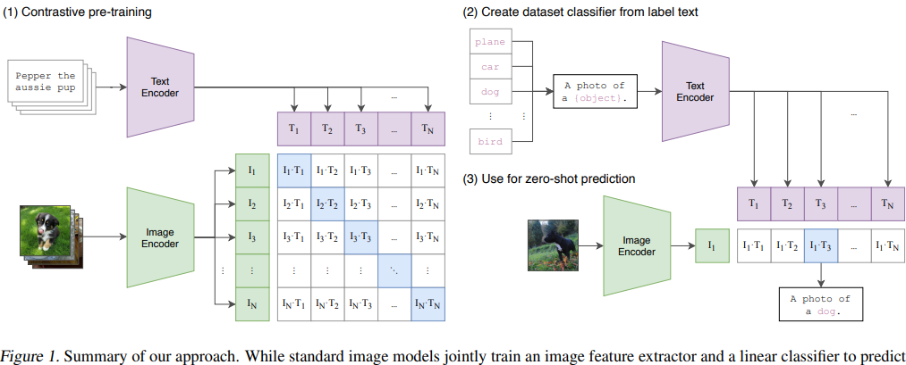
<p align="center">
  <img src="/assets/img/clip_architecture.png" width="100%" />
</p>

<p>CLIP learns aligned image and text representations through contrastive learning. Instead of predicting fixed class labels, CLIP learns aligned image-text embeddings with a contrastive loss:</p>

\[L_{\text{CLIP}}
=
-\frac1N
\sum_i
\log
\frac{
\exp(\text{sim}(f(x_i),g(t_i))/\tau)
}{
\sum_j
\exp(\text{sim}(f(x_i),g(t_j))/\tau)
}\]

<p>Instead of class labels $y\in{1,\ldots,K}$, CLIP produces a semantic conditioning vector</p>

\[c=g(\text{prompt})\]

<p>which later becomes the text condition used in diffusion.</p>

<h3 id="core-contribution-1">Core contribution</h3>

<p>The important shift introduced by CLIP was replacing fixed-label supervision with natural language supervision at internet scale. Instead of learning closed-set classification boundaries, CLIP learned a shared semantic embedding space between images and text. This later became the conditioning interface for modern diffusion models:</p>

\[c = f_{text}(\text{prompt})\]

<p>where text embeddings guide image generation through cross-attention and CFG-based sampling. CLIP therefore became one of the key foundations of prompt-conditioned generative systems and modern multimodal models.</p>

<h2 id="5-classifier-free-guidance-cfg">5. Classifier-Free Guidance (CFG)</h2>

<p>CFG becomes much easier to understand when viewed as a continuation of the probabilistic framework introduced by VAE and DDPM.</p>

<p>VAE introduced variational optimization through the ELBO:</p>

\[\log p(x)
\geq
\mathbb{E}_{q(z|x)}[\log p(x|z)]

- D_{KL}(q(z|x)||p(z))\]

<p>DDPM inherited this probabilistic viewpoint and derived a variational objective over the diffusion trajectory which was later simplified into the practical denoising objective:</p>

\[L_{simple}
=
\mathbb{E}_{x_0,\epsilon,t}
\left[
||
\epsilon
-
\epsilon_\theta(x_t,t)
||^2
\right]\]

<p>CFG extends this same denoising framework into conditional generation by training both:</p>

\[\epsilon_\theta(x_t,t,c),
\quad
\epsilon_\theta(x_t,t)\]

<p>through random condition dropping. Sampling then combines conditional and unconditional predictions:</p>

\[\hat{\epsilon}_\theta(z_t,c)

= (1+w)\epsilon_\theta(z_\lambda,c)
-
w\epsilon_\theta(z_t)\]

<p>where the residual term isolates the conditional signal introduced by the prompt. Earlier diffusion systems relied on external classifier gradients for guidance, but CFG removed this requirement entirely while dramatically improving prompt alignment. This simple modification became one of the most important practical advances in modern diffusion models.</p>

<h2 id="6-masked-autoencoder-mae">6. Masked Autoencoder (MAE)</h2>

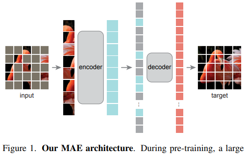
<p align="center">
  <img src="/assets/img/mae.png" width="100%" />
</p>

<p>MAE performs self-supervised learning by masking a large portion of image patches and reconstructing the missing content from only the visible patches. Unlike earlier reconstruction-based methods, the encoder processes only unmasked tokens while reconstruction is delegated to a lightweight decoder, making training substantially more efficient despite very high masking ratios. This showed that transformer-based vision models could learn strong semantic representations directly from unlabeled data and significantly strengthened the ViT ecosystem. More broadly, MAE helped establish transformers as scalable visual backbones, indirectly accelerating later transformer-based generative systems such as DiT.</p>

<h2 id="7-latent-diffusion-models-ldm">7. Latent Diffusion Models (LDM)</h2>

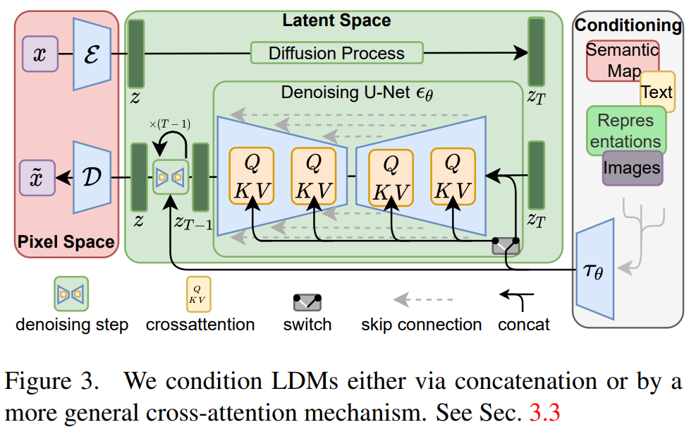
<p align="center">
  <img src="/assets/img/LDM.png" width="100%" />
</p>

<p>LDM compresses images into a learned latent space through an autoencoder:</p>

\[z=\mathcal{E}(x),
\qquad
x=\mathcal{D}(z)\]

<p>and performs diffusion directly on latent representations rather than pixel-space tensors. Importantly, the training objective remains almost identical to DDPM:</p>

\[L_{\text{DDPM}}\mathbb{E}\left[|\epsilon-\epsilon_\theta(x_t,t)|^2\right]

\qquad

L_{\text{LDM}}\mathbb{E}\left[|\epsilon-\epsilon_\theta(z_t,t,c)|^2\right]\]

<p>with the primary structural change being:</p>

\[x_t \rightarrow z_t\]

<p>This substantially reduces computational cost by moving diffusion onto a lower-dimensional manifold while preserving high perceptual quality. Conditioning is introduced through CLIP text embeddings:</p>

\[c=f_{\text{text}}(\text{prompt})\]

<p>and sampling is guided using CFG:</p>

\[\hat\epsilon_\theta

\epsilon_\theta(z_t,t)
+
w\Big(
\epsilon_\theta(z_t,t,c)

\epsilon_\theta(z_t,t)
\Big)\]

<p>Conceptually, LDM can be viewed as the convergence of several earlier developments:</p>

\[\text{VAE}
+
\text{DDPM}
+
\text{CLIP}
+
\text{CFG}\]

<p>This combination transformed diffusion models from computationally expensive research systems into practical large-scale text-to-image generators and later became the foundation of Stable Diffusion.</p>

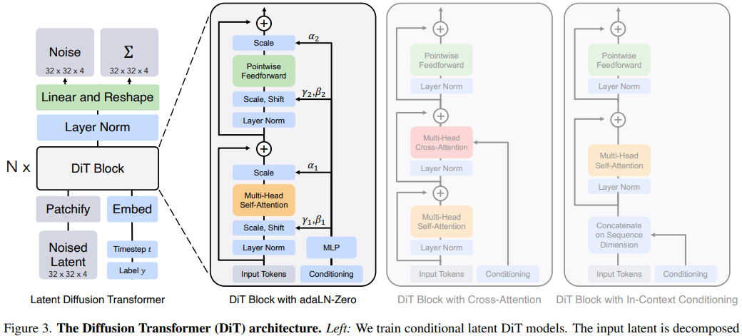
<h2 id="8-diffusion-transformer-dit">8. Diffusion Transformer (DiT)</h2>

<p align="center">
  <img src="/assets/img/dit_architecture.png" width="100%" />
</p>

<p>Earlier diffusion systems mainly used convolutional U-Nets as denoising backbones. DiT replaced this architecture with transformers operating directly on latent patches. DiT replaces the U-Net denoiser with a transformer over latent patches:</p>

\[z\rightarrow\{z_p^1,\ldots,z_p^N\}\]

<p>with the same attention rule used in ViT:</p>

\[\text{Attention}(Q,K,V)
=
\text{softmax}\!\left(\frac{QK^T}{\sqrt d}\right)V\]

<p>The diffusion loss is unchanged in form:</p>

\[L_{\text{DiT}}
=
\mathbb{E}
\left[
\|\epsilon-\epsilon_\theta(z_t,t,c)\|^2
\right]\]

<p>The architectural change is</p>

\[\text{U-Net}\rightarrow\text{Transformer}\]

<p>so DiT keeps the diffusion objective while swapping in a transformer backbone.</p>

<h3 id="core-contribution-2">Core contribution</h3>

<p>DiT replaced convolutional U-Nets with transformer-based diffusion backbones operating on latent patches while preserving the standard diffusion objective.</p>

<p>The key result was that diffusion models inherit transformer scaling behavior: performance improves predictably with model size, training compute, and dataset scale. DiT accelerated the transition toward transformer-native generative systems and strongly influenced later work in video generation, multimodal generation, and world models.</p>

<h2 id="whats-next">What’s Next?</h2>

<h3 id="1-multimodal-models">1. Multimodal models</h3>

<p>Modern systems jointly model text, images, video, audio, and actions. Representative works include GPT-4o, which unifies multimodal interaction inside a single model.</p>

<ul>
  <li>OpenAI. (2024). <strong>Hello GPT-4o</strong>. <em>OpenAI.</em>
<a href="https://openai.com/index/hello-gpt-4o/">https://openai.com/index/hello-gpt-4o/</a></li>
</ul>

<h3 id="2-video-generation">2. Video generation</h3>

<p>Image generation is rapidly extending into video generation, where the central challenges are temporal consistency, motion understanding, and world simulation. A representative example is Sora, which applies diffusion transformers to large-scale video generation.</p>

<ul>
  <li>OpenAI. (2024). <strong>Video generation models as world simulators</strong>. <em>OpenAI.</em>
<a href="https://openai.com/research/video-generation-models-as-world-simulators">https://openai.com/research/video-generation-models-as-world-simulators</a></li>
</ul>

<h3 id="3-faster-diffusion-methods">3. Faster diffusion methods</h3>

<p>Although diffusion models produce high-quality outputs, sampling remains expensive. Current research focuses on reducing sampling steps through methods such as Flow Matching, which reformulates generative modeling through continuous probability flows.</p>

<ul>
  <li>Lipman, Y., Chen, R. T. Q., Ben-Hamu, H., Nickel, M., &amp; Le, M. (2022). <strong>Flow matching for generative modeling</strong>. <em>arXiv preprint arXiv:2210.02747.</em>
<a href="https://arxiv.org/abs/2210.02747">https://arxiv.org/abs/2210.02747</a></li>
</ul>

<h3 id="4-world-models">4. World models</h3>

<p>The field is increasingly focused not only on visual quality, but also on reasoning, physical consistency, interaction, and long-horizon generation. One influential direction is Genie, which explores generative interactive world models for agents and simulation.</p>

<ul>
  <li>Bruce, J., et al. (2024). <strong>Genie: Generative interactive environments</strong>. <em>arXiv preprint arXiv:2402.15391.</em>
<a href="https://arxiv.org/abs/2402.15391">https://arxiv.org/abs/2402.15391</a></li>
</ul>

<h2 id="final-thoughts">Final Thoughts</h2>

<p>How naturally these papers connect into a single generative framework is truly beautiful. Each work extends and reuses ideas introduced by the previous ones. VAE introduced latent-variable inference and variational optimization. DDPM reformulated generation into probabilistic diffusion modeling. ViT and MAE showed that transformers could outperform previous convolutional architectures while introducing scaling behavior into vision. CLIP transformed natural language into a semantic conditioning interface, CFG made diffusion models practically controllable, and LDM unified these developments into an efficient latent-space generative system. Finally, DiT demonstrated that transformer scaling laws extend directly into diffusion-based image generation itself.</p>

<p>After reading these 8 papers, I hope you can feel how modern generative AI emerged not from a single breakthrough, but from the gradual convergence of the concepts introduced by them. It is a beautiful journey: as you move from one paper to the next, concepts, equations, and architectural decisions continuously resurface in new forms. Recognizing where those ideas originated—and seeing how later systems inherit and build upon them—brings a surprising sense of coherence and joy to whoever is trying to - or is already in - the field of computer vision.</p>

<h2 id="references">References</h2>

<ol>
  <li>Kingma, D. P., &amp; Welling, M. (2013). <strong>Auto-encoding variational bayes</strong>. <em>arXiv preprint arXiv:1312.6114.</em>
 <a href="https://arxiv.org/abs/1312.6114">https://arxiv.org/abs/1312.6114</a></li>
  <li>Ho, J., Jain, A., &amp; Abbeel, P. (2020). <strong>Denoising diffusion probabilistic models</strong>. <em>Advances in Neural Information Processing Systems, 33.</em>
<a href="https://arxiv.org/abs/2006.11239">https://arxiv.org/abs/2006.11239</a></li>
  <li>Dosovitskiy, A., Beyer, L., Kolesnikov, A., Weissenborn, D., Zhai, X., Unterthiner, T., Dehghani, M., Minderer, M., Heigold, G., Gelly, S., Uszkoreit, J., &amp; Houlsby, N. (2020). <strong>An image is worth 16x16 words: Transformers for image recognition at scale</strong>. <em>arXiv preprint arXiv:2010.11929.</em>
<a href="https://arxiv.org/abs/2010.11929">https://arxiv.org/abs/2010.11929</a></li>
  <li>Radford, A., Kim, J. W., Hallacy, C., Ramesh, A., Goh, G., Agarwal, S., Sastry, G., Askell, A., Mishkin, P., Clark, J., Krueger, G., &amp; Sutskever, I. (2021). <strong>Learning transferable visual models from natural language supervision</strong>. <em>Proceedings of the 38th International Conference on Machine Learning.</em>
<a href="https://arxiv.org/abs/2103.00020">https://arxiv.org/abs/2103.00020</a></li>
  <li>Ho, J., &amp; Salimans, T. (2021). <strong>Classifier-free diffusion guidance</strong>. <em>arXiv preprint arXiv:2207.12598.</em>
<a href="https://arxiv.org/abs/2207.12598">https://arxiv.org/abs/2207.12598</a></li>
  <li>He, K., Chen, X., Xie, S., Li, Y., Dollár, P., &amp; Girshick, R. (2021). <strong>Masked autoencoders are scalable vision learners</strong>. <em>Proceedings of the IEEE/CVF Conference on Computer Vision and Pattern Recognition (CVPR).</em>
<a href="https://arxiv.org/abs/2111.06377">https://arxiv.org/abs/2111.06377</a></li>
  <li>Rombach, R., Blattmann, A., Lorenz, D., Esser, P., &amp; Ommer, B. (2022). <strong>High-resolution image synthesis with latent diffusion models</strong>. <em>Proceedings of the IEEE/CVF Conference on Computer Vision and Pattern Recognition (CVPR).</em>
<a href="https://arxiv.org/abs/2112.10752">https://arxiv.org/abs/2112.10752</a></li>
  <li>Peebles, W., &amp; Xie, S. (2022). <strong>Scalable diffusion models with transformers</strong>. <em>Proceedings of the IEEE/CVF International Conference on Computer Vision (ICCV).</em>
<a href="https://arxiv.org/abs/2212.09748">https://arxiv.org/abs/2212.09748</a></li>
</ol>

<h2 id="written-by">Written by</h2>
<blockquote>
  <p><strong>Roger Kim</strong><br />
<a href="https://github.com/kmsrogerkim"><img src="https://img.shields.io/badge/GitHub-181717?logo=github&amp;logoColor=white" alt="GitHub" /></a> <a href="https://www.linkedin.com/in/kmsrogerkim/"><img src="https://img.shields.io/badge/LinkedIn-0A66C2?logo=linkedin&amp;logoColor=white" alt="LinkedIn" /></a></p>
</blockquote>]]></content><author><name>Roger Kim</name></author><category term="AI" /><category term="AI" /><category term="CV" /><summary type="html"><![CDATA[Here are 8 essential computer vision papers I read that forms the foundation of modern computer vision / generative models; in chronological order.]]></summary></entry><entry><title type="html">Understanding CvT: Introducing Convolutions to Vision Transformers</title><link href="https://kmsrogerkim.github.io/ai/cvt/" rel="alternate" type="text/html" title="Understanding CvT: Introducing Convolutions to Vision Transformers" /><published>2025-08-19T00:00:00+00:00</published><updated>2025-08-19T00:00:00+00:00</updated><id>https://kmsrogerkim.github.io/ai/cvt</id><content type="html" xml:base="https://kmsrogerkim.github.io/ai/cvt/"><![CDATA[<h2 id="convolutional-vision-transformer-cvt-introducing-convolutions-to-vision-transformers">Convolutional Vision Transformer (CvT): Introducing Convolutions to Vision Transformers</h2>

<p>In 2021, Vision Transformer (ViT) showed us that Transformers could be used to solve vision tasks. With <strong>deep enough models</strong> and <strong>big enough data</strong>, ViT outperformed previous SOTA models.</p>

<blockquote>
  <p>However, the paper (Dosovitskiy et al., 2021) made it very clear that ViTs lack CNNs’ inductive bias, thus the data-hungry nature of ViTs.</p>
</blockquote>

<p>Well then, somebody must have thought of a way to integrate the inductive bias of CNNs into ViTs, right?</p>

<p>That’s how the <strong>Convolutional Vision Transformer (CvT)</strong> was born (Wu et al., 2021).</p>

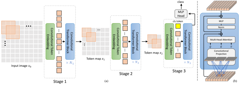
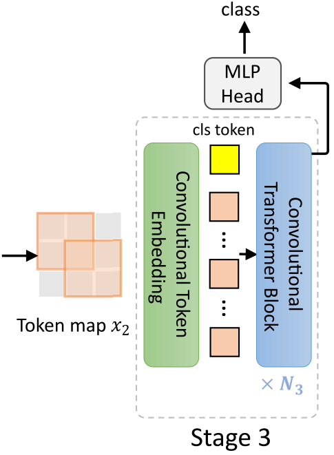
<h2 id="architecture-overview">Architecture Overview</h2>

<p align="center">
  <img src="/assets/img/cvt/cvt_architecture.png" width="100%" />
</p>

<p>CvT follows a <strong>multi-stage hierarchical design</strong>, inspired by CNNs:</p>

<ul>
  <li><strong>Stage 1</strong>:<br />
The input image is first processed by a <strong>Convolutional Token Embedding</strong> layer.
    <ul>
      <li>Unlike ViT’s fixed patch embedding, CvT uses <strong>overlapping convolutions</strong>, which preserve local spatial information.</li>
      <li>This produces the first <strong>token map</strong> $x_1$, which then passes through several <strong>Convolutional Transformer Blocks</strong>.</li>
    </ul>
  </li>
  <li><strong>Stage 2</strong>:<br />
Another <strong>Convolutional Token Embedding</strong> downsamples and expands the representation, reducing the number of tokens while increasing feature richness.
    <ul>
      <li>The new token map $x_2$ again flows through Transformer blocks.</li>
    </ul>
  </li>
  <li><strong>Stage 3</strong>:<br />
Further downsampling into a compact token map $x_3$. Then, CLS token is added before the token map is fed into the CvT block.
    <ul>
      <li>The output is passed through an <strong>MLP head</strong> to produce the final prediction.</li>
    </ul>
  </li>
</ul>

<h3 id="important-details">Important Details</h3>
<ol>
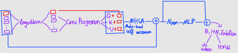
  <li>cls token bypasses convolution projection and is reinserted before MHSA.</li>
  <li>Each stage is repeated $N_n$ times.</li>
  <li>Remember to add padding according to your kernel size.</li>
  <li>Size of K&amp;V may differ from Q depending on your choice of convolutional projection</li>
  <li>Stride of the convolutional token embadding is explicitly defined in the paper for each model.</li>
</ol>

<h2 id="convolutional-token-embedding">Convolutional Token Embedding</h2>

<p>The <strong>Convolutional Token Embedding</strong> layer is CvT’s replacement for ViT’s patch embedding. Its goal is to model <strong>local spatial context</strong>. From low-level edges and textures to higher-order semantic patterns; while building a <strong>hierarchical representation.</strong></p>

<ul>
  <li>Instead of splitting an image into <strong>non-overlapping patches</strong> (as ViT does), CvT applies an <strong>overlapping convolution</strong>.</li>
  <li>This helps preserve neighboring relationships between pixels .</li>
  <li>At each stage, the convolution <strong>reduces the token sequence length</strong> while <strong>increasing feature dimensionality</strong>:
    <ul>
      <li>Fewer tokens → more compact representations.</li>
      <li>Richer features → higher-level semantics captured.</li>
    </ul>
  </li>
  <li>After convolution, the token map is <strong>flattened and normalized</strong> before being fed into Transformer blocks.</li>
</ul>

<p>Formally,</p>
<ul>
  <li>given the token map from the previous stage</li>
</ul>

\[x_{i-1} \in \mathbb{R}^{H_{i-1} \times W_{i-1} \times C_{i-1}}\]

<ul>
  <li>a 2D convolution with kernel size $s \times s$, stride $s - o$, and padding $p$ produces a new token map</li>
</ul>

\[f(x_{i-1}) \in \mathbb{R}^{H_i \times W_i \times C_i}\]

<ul>
  <li>which has the height and width of:</li>
</ul>

\[H_i = \left\lfloor \frac{H_{i-1} + 2p - s}{s - o} + 1\right\rfloor\]

\[W_i = \left\lfloor \frac{W_{i-1} + 2p - s}{s - o} + 1\right\rfloor\]

<p>$f(x_{i−1})$ is then flattened into size $H_i W_i × C_i$ and passed through a layer normalization.</p>

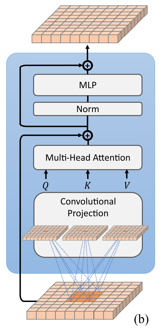
<h2 id="convolutional-transformer-block">Convolutional Transformer Block</h2>

<p align="center">
  <img src="/assets/img/cvt/cvt_block.png" width="90%" />
</p>

<ul>
  <li>In ViT, queries/keys/values are projected linearly.</li>
  <li>CvT replaces these with <strong>depth-wise separable convolutions</strong>.</li>
  <li>This lets attention look at <strong>local neighborhoods</strong> before going global, improving efficiency and reducing ambiguity.</li>
</ul>

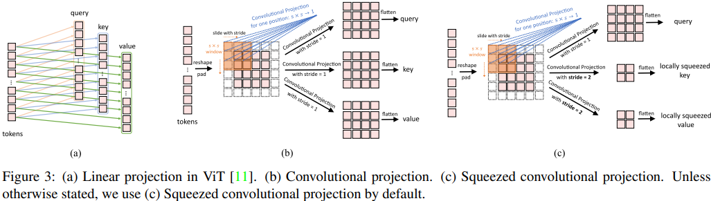
<h3 id="convolutional-projection">Convolutional Projection</h3>

<p align="center">
  <img src="/assets/img/cvt/cvt_projection.png" width="100%" />
</p>

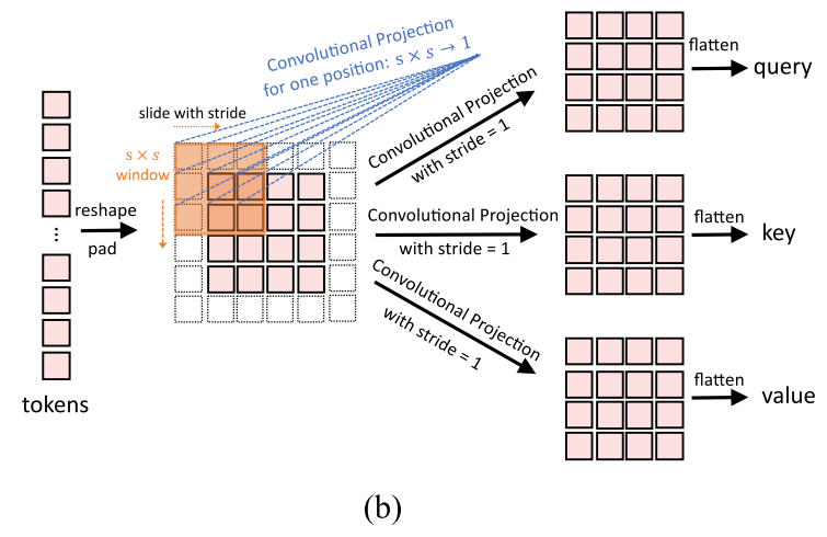
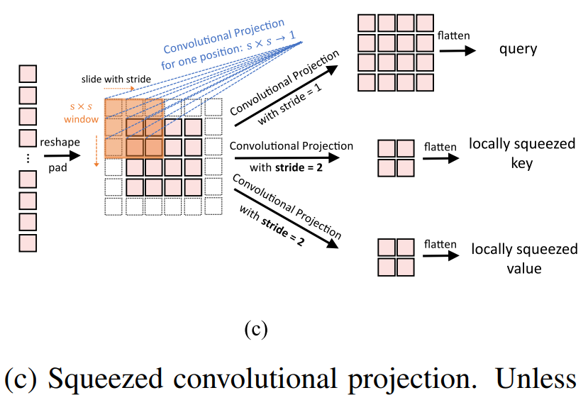
<p>“The goal of the proposed Convolutional Projection layer is to achieve additional modeling of local spatial context, and to provide efficiency benefits by permitting the undersampling of K and V matrices” (Wu et al., 2021).</p>

<p>Now, you have to be careful when implementing CvT, since the paper states that they use <strong>squeezed</strong> convolutional projection by default.</p>

<p align="center">
  <img src="/assets/img/cvt/normal_cvt_projection.png" width="100%" />
</p>

<h3 id="convolutional-projection-1">Convolutional Projection</h3>
<ul>
  <li>Replaces ViT’s linear Q/K/V with <strong>depthwise separable convolutions</strong> (stride = 1).</li>
  <li>Preserves full resolution for Q, K, V.</li>
</ul>

<p align="center">
  <img src="/assets/img/cvt/squeezed_convolutional_projection.png" width="100%" />
</p>

<h3 id="squeezed-convolutional-projection">Squeezed Convolutional Projection</h3>
<ul>
  <li>Uses <strong>stride = 1</strong> for Q, but <strong>stride = 2</strong> for K and V (downsampled).</li>
  <li>Cuts K/V tokens by 4×, reducing MHSA cost.</li>
  <li><strong>Benefit</strong>: ~30% fewer FLOPs, <strong>almost</strong> no accuracy loss.</li>
</ul>

<blockquote>
  <p>Keep in mind that the paper uses squeezed convolutional projection by default.</p>
</blockquote>

<h2 id="cls-token-in-stage-3">CLS Token in Stage 3</h2>

<p align="center">
  <img src="/assets/img/cvt/cls_token1.png" width="90%" />
</p>

<p>For CvTs, cls token is not added until stage 3. I will explain it in detail how cls token is passed through in each layer in stage 3. This could be a little pain in the ass when implementing.</p>

<p align="center">
  <img src="/assets/img/cvt/cls_token2.png" width="100%" />
</p>

<ol>
  <li>The entire input vector goes through layer normalization.</li>
  <li>cls token is seperated</li>
  <li>The rest (spatial patches) goes through (squeezed) convolutional projection, generating Q,K,V</li>
  <li>cls token is concatenated back, and passed through multi-head attention layer</li>
  <li>Rest follows the standard transformer pattern</li>
</ol>

<h2 id="results">Results</h2>

<p align="center">
  <img src="/assets/img/cvt/cvt_models.png" width="100%" />
</p>

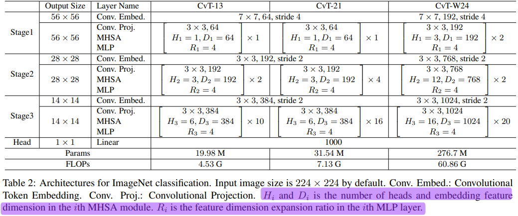
<p>Thankfully, the paper provided detailed architecture of each CvT model they used for training. You can go ahead and implement the model right now!</p>

<p>On <strong>ImageNet-1k</strong>:</p>
<ul>
  <li>CvT-21 reaches <strong>82.5% top-1 accuracy</strong>, outperforming DeiT-B with <strong>63% fewer parameters</strong> and <strong>60% fewer FLOPs</strong>.</li>
  <li>Even the smaller CvT-13 (20M params) beats ResNet-152, which has 3× more parameters.</li>
</ul>

<p>On <strong>ImageNet-22k (pretraining)</strong> → fine-tuned to ImageNet-1k:</p>
<ul>
  <li>CvT-W24 scores <strong>87.7% top-1</strong>, surpassing ViT-L/16 by <strong>+2.5%</strong>, without using extra datasets like JFT-300M.</li>
</ul>

<p>On <strong>transfer tasks</strong> (CIFAR, Oxford Flowers, Pets):</p>
<ul>
  <li>CvT consistently outperforms both ViTs and ResNets, showing strong generalization.</li>
</ul>

<h2 id="code-implementation">Code Implementation</h2>

<ul>
  <li>My PyTroch implementation:
    <ul>
      <li><a href="https://github.com/kmsrogerkim/CvT-PyTorch">https://github.com/kmsrogerkim/CvT-PyTorch</a></li>
    </ul>
  </li>
  <li>Official Microsoft implementation:
    <ul>
      <li><a href="https://github.com/microsoft/CvT">https://github.com/microsoft/CvT</a></li>
    </ul>
  </li>
</ul>

<h2 id="final-thoughts">Final Thoughts</h2>

<p>CvT is a clever hybrid.</p>
<blockquote>
  <p>it <strong>keeps the scalability and global reasoning of Transformers</strong>, but regains the <strong>local structure and efficiency of CNNs</strong>.</p>
</blockquote>

<ul>
  <li>ViTs taught us that <strong>scale wins</strong>.</li>
  <li>CvT shows that <strong>inductive bias still matters</strong> — and when used strategically, it makes Transformers more data-efficient, lightweight, and robust.</li>
</ul>

<h2 id="references">References</h2>

<ol>
  <li>
    <p>Wu, H., Xiao, B., Codella, N., Liu, M., Dai, X., Yuan, L., &amp; Zhang, L. (2021). <strong>CvT: Introducing Convolutions to Vision Transformers.</strong> <em>arXiv preprint arXiv:2103.15808.</em><br />
<a href="https://arxiv.org/abs/2103.15808">https://arxiv.org/abs/2103.15808</a></p>
  </li>
  <li>
    <p>Dosovitskiy, A., Beyer, L., Kolesnikov, A., Weissenborn, D., Zhai, X., Unterthiner, T., … &amp; Houlsby, N. (2021). <strong>An image is worth 16x16 words: Transformers for image recognition at scale.</strong> <em>ICLR.</em><br />
<a href="https://arxiv.org/abs/2010.11929">https://arxiv.org/abs/2010.11929</a></p>
  </li>
</ol>

<h2 id="written-by">Written by</h2>
<blockquote>
  <p><strong>Roger Kim</strong><br />
<a href="https://github.com/kmsrogerkim"><img src="https://img.shields.io/badge/GitHub-181717?logo=github&amp;logoColor=white" alt="GitHub" /></a> <a href="https://www.linkedin.com/in/kmsrogerkim/"><img src="https://img.shields.io/badge/LinkedIn-0A66C2?logo=linkedin&amp;logoColor=white" alt="LinkedIn" /></a></p>
</blockquote>]]></content><author><name>Roger Kim</name></author><category term="AI" /><category term="AI" /><category term="CV" /><summary type="html"><![CDATA[Convolutional Vision Transformer (CvT): Introducing Convolutions to Vision Transformers]]></summary></entry><entry><title type="html">ViT: AN IMAGE IS WORTH 16X16 WORDS</title><link href="https://kmsrogerkim.github.io/ai/vit/" rel="alternate" type="text/html" title="ViT: AN IMAGE IS WORTH 16X16 WORDS" /><published>2025-08-18T00:00:00+00:00</published><updated>2025-08-18T00:00:00+00:00</updated><id>https://kmsrogerkim.github.io/ai/vit</id><content type="html" xml:base="https://kmsrogerkim.github.io/ai/vit/"><![CDATA[<h2 id="vision-transformer-vit-an-image-is-worth-16x16-words">Vision Transformer (ViT): AN IMAGE IS WORTH 16X16 WORDS</h2>

<p>For decades, CNNs dominated computer vision. From <strong>LeNet</strong> to <strong>ResNet</strong>, convolution and locality were treated as fundamental building blocks.</p>

<p>But in 2021, researchers at <strong>Google Brain</strong> challenged this assumption. They asked a bold question:</p>

<blockquote>
  <p>Could we throw away convolutions and use <em>only</em> Transformers?</p>
</blockquote>

<p>The answer was yes—if with <strong>enough</strong> data. Their paper <em>“An Image is Worth 16x16 Words: Transformers for Image Recognition at Scale”</em> introduced the <strong>Vision Transformer (ViT)</strong>, a model that treats images like sequences of word tokens, and achieves <strong>state-of-the-art accuracy</strong> on large-scale image classification.</p>

<h2 id="an-image-is-worth-16x16-words">An Image is Worth 16x16 Words</h2>
<p>Here’s how images are fed into ViTs</p>

<ul>
  <li>First, we slice an image into fixed-size <strong>patches</strong> (16×16 in this paper).</li>
  <li>Each patch is <strong>flattened into a vector</strong> and <strong>linearly projected</strong>.</li>
  <li>These patch embeddings are treated exactly like <strong>tokens in NLP</strong>.</li>
  <li>The <strong>cls token</strong> is added to represent the image’s classification output.</li>
  <li>Then the <strong>positional embeddings</strong> are added.</li>
</ul>

<p>Mathematically, if an image has resolution $(H, W)$ and $C$ channels, patches of size $(P, P)$ yield:</p>

\[N = \frac{H \cdot W}{P^2}\]

<p>patches, which form the Transformer input sequence.</p>

<p>So you can see how the paper came up with the title <em>“An Image is Worth 16x16 Words”</em>. Just like how strings were tokenized and embedded, an image is now split into patches and embedded, then fed to Transformer encoder.</p>

<h2 id="architecture-overview">Architecture Overview</h2>

<p align="center">
  <img src="/assets/img/vit/vit_architecture.png" width="100%" />
</p>

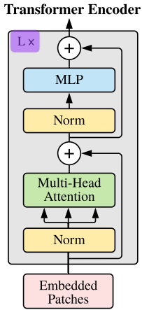
<p>ViT keeps the original Transformer encoder design. Let’s look at how the model works through some simple equations presented in the paper</p>

<h3 id="1-input-sequence-construction">(1): Input Sequence Construction</h3>

\[z_0 = [x_{class}; x_p^1E; x_p^2E; \dots; x_p^N E] + E_{pos}\]

<ul>
  <li><strong>$x_p^i \quad$</strong>: the $i$-th image patch (flattened)</li>
  <li><strong>$E \quad $</strong>: the patch-embedding projection matrix</li>
  <li><strong>$E_{pos}$</strong>: the positional embedding</li>
  <li><strong>$x_{class}$</strong>: the <strong>classification token</strong></li>
  <li><strong>$z_0 \quad$</strong>: the full <strong>input sequence to the Transformer encoder</strong>, consisting of:
    <ul>
      <li>1 classification token</li>
      <li>$N$ patch embeddings</li>
      <li>plus positional encodings</li>
    </ul>
  </li>
</ul>

<h3 id="2-3-transformer-encoder-layers">(2), (3): Transformer Encoder Layers</h3>

<p align="center">
  <img src="/assets/img/vit/transformer_encoder.png" width="30%" />
</p>

\[z'_\ell = MSA(LN(z_{\ell-1})) + z_{\ell-1}\]

\[z_\ell = MLP(LN(z'_\ell)) + z'_\ell\]

<p>This repeats for $L$ layers.</p>

<h3 id="4-final-representation">(4): Final Representation</h3>

\[y = LN(z_L^0)\]

<ul>
  <li>$z_L$: the sequence after the final ($L$-th) Transformer block.</li>
  <li>$z_L^0$: the <strong>first token</strong> (the [CLS] token).</li>
  <li>$y$: the final output, passed through the MLP head for classfication.</li>
</ul>

<h3 id="in-short">In short:</h3>
<ol>
  <li>The image is turned into a sequence ($z_0$), which includes patch + positional embedding, and <em>extra learnable [class] embedding</em></li>
  <li>Processed layer by layer through transformer encoder, finally outputting ($z_\ell$)</li>
  <li>Then the first token of the $z_\ell$, $z_\ell^0$ (the cls token) is passed through a layer normalization layer outputting $y$</li>
  <li>Finally $y$ is passed through a 2-layer MLP head(pre-training), or a linear classifier(fine-tuning).</li>
</ol>

<h2 id="scale-over-inductive-bias">Scale Over Inductive Bias</h2>

<p>The paper clearly noted that ViTs have far less image-specific inductive bias than CNNs.</p>

<ul>
  <li>In CNNs, properties like <strong>locality</strong>, <strong>two-dimensional neighborhood structure</strong>, and <strong>translation equivariance</strong> are baked into every layer. Convolutions naturally capture local pixel patterns and preserve spatial hierarchies.</li>
  <li>In ViTs, the <strong>self-attention layers</strong> are <strong>global</strong> by design: every patch can attend to every other patch, regardless of distance.</li>
  <li>The <strong>MLP layers</strong> are <strong>position-wise</strong> (applied independently to each token), which makes them translation-equivariant at the token level, but they do not capture local pixel neighborhoods the way convolutions do.</li>
  <li>The <strong>2D structure</strong> is used only twice:
    <ul>
      <li>At the start, by cutting the image into patches.</li>
      <li>At fine-tuning time, when adjusting positional embeddings for different resolutions.</li>
    </ul>
  </li>
  <li>Aside from this, the <strong>positional embeddings</strong> contain no explicit 2D spatial information. This means <strong>all spatial relations between patches must be learned from scratch</strong>.</li>
</ul>

<p>This design explains why ViTs underperform CNNs on smaller datasets but excel once scaled to large data and model sizes.</p>

<h2 id="model-size--dataset-size">Model Size &amp; Dataset Size</h2>

<p align="center">
  <img src="/assets/img/vit/vit_variants.png" width="90%" />
</p>

<ul>
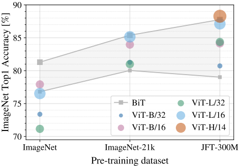
  <li>On small datasets (like ImageNet-1k), ViTs underperform compared to CNNs</li>
  <li>On ImageNet-21k, ViTs and ResNet performed similarly.</li>
  <li>Only after pre-training with the JFT-300M dataset ViTs HUGE model <strong>outperformed.</strong></li>
</ul>

<p align="center">
  <img src="/assets/img/vit/dataset_size_graph.png" width="90%" />
</p>

<blockquote>
  <p>The pros and cons have become very clear at this point.</p>
</blockquote>

<p>Since ViTs lack the image-specific inductive bias that CNNs possess, they underperform on small datasets. However, with huge dataset and models that are deep enough (632M parameters), they can outperform current SOTA image classification models; even with its simple and straight forward architecture.</p>

<h2 id="self-supervision">Self-Supervision</h2>
<p>One of the key drivers of Transformers’ success in NLP was not just the architecture itself, but <strong>large-scale self-supervised pre-training</strong>. Models like <strong>BERT</strong> (Devlin et al., 2019) and <strong>GPT</strong> (Radford et al., 2018) learned powerful representations by predicting masked words or the next word in a sentence — allowing them to leverage massive amounts of unlabeled text.</p>

<p>The ViT paper explores whether a similar strategy can help in computer vision.</p>

<h3 id="masked-patch-prediction">Masked Patch Prediction</h3>

<p>To mimic BERT’s <strong>masked language modeling</strong>, ViT applies <strong>masked patch prediction</strong>:</p>

<ul>
  <li>During training, some image patches are <strong>masked out</strong> (hidden from the model).</li>
  <li>The model is trained to <strong>predict the embeddings</strong> of the missing patches from the visible ones.</li>
  <li>This encourages the Transformer to learn <strong>semantic relationships between patches</strong>, much like how BERT learns contextual relationships between words.</li>
</ul>

<p>*<em>Unlike later approaches such as <strong>MAE</strong> (He et al., 2022) or <strong>BEiT</strong> (Bao et al., 2021), the original ViT did not attempt to reconstruct raw pixel values. Instead, it focused on predicting patch embeddings.</em></p>

<p>Anyways the paper tried the masked patch prediction with the <strong>ViT-B/16</strong> model and got:</p>
<ul>
  <li><strong>79.9%</strong> accuracy on ImageNet, which is about a <strong>2% improvement</strong> over training from scratch</li>
  <li>though still around 4% lower than results from supervised pre-training.</li>
</ul>

<h2 id="final-thoughts">Final Thoughts</h2>
<p>With deep enough models and big enough data, ViT outperforms previous SOTA models. The paper made it very clear that ViTs lack CNNs’ inductive bias, thus the data-hungry nature of ViTs.</p>

<p>Well then, somebody must have thought of a way to integrate the inductive bias of CNNs into ViTs, right? That’s why I am also going to review <em>CvT: Introducing Convolutions to Vision Transformers</em>.</p>

<p>So…tune in for the next blog post! See you around.</p>

<h2 id="references">References</h2>
<ol>
  <li>Bao, H., Dong, L., &amp; Wei, F. (2021). <strong>BEiT: BERT Pre-Training of Image Transformers.</strong> <em>arXiv preprint arXiv:2106.08254.</em><br />
  <a href="https://arxiv.org/abs/2106.08254">https://arxiv.org/abs/2106.08254</a></li>
  <li>Dosovitskiy, A., Beyer, L., Kolesnikov, A., Weissenborn, D., Zhai, X., Unterthiner, T., … &amp; Houlsby, N. (2021). <strong>An image is worth 16x16 words: Transformers for image recognition at scale.</strong> <em>International Conference on Learning Representations (ICLR).</em><br />
  <a href="https://arxiv.org/abs/2010.11929">https://arxiv.org/abs/2010.11929</a></li>
  <li>He, K., Chen, X., Xie, S., Li, Y., Dollár, P., &amp; Girshick, R. (2022). <strong>Masked Autoencoders Are Scalable Vision Learners.</strong> <em>Proceedings of the IEEE/CVF Conference on Computer Vision and Pattern Recognition (CVPR)</em>, 16000–16009. 
  <a href="https://arxiv.org/abs/2111.06377">https://arxiv.org/abs/2111.06377</a></li>
</ol>

<h2 id="written-by">Written by</h2>
<blockquote>
  <p><strong>Roger Kim</strong><br />
<a href="https://github.com/kmsrogerkim"><img src="https://img.shields.io/badge/GitHub-181717?logo=github&amp;logoColor=white" alt="GitHub" /></a> <a href="https://www.linkedin.com/in/kmsrogerkim/"><img src="https://img.shields.io/badge/LinkedIn-0A66C2?logo=linkedin&amp;logoColor=white" alt="LinkedIn" /></a></p>
</blockquote>]]></content><author><name>Roger Kim</name></author><category term="AI" /><category term="AI" /><category term="CV" /><summary type="html"><![CDATA[Vision Transformer (ViT): AN IMAGE IS WORTH 16X16 WORDS]]></summary></entry><entry><title type="html">Evolution of Multiple Object Detection and the Rise of YOLO</title><link href="https://kmsrogerkim.github.io/ai/yolo/" rel="alternate" type="text/html" title="Evolution of Multiple Object Detection and the Rise of YOLO" /><published>2025-08-17T00:00:00+00:00</published><updated>2025-08-17T00:00:00+00:00</updated><id>https://kmsrogerkim.github.io/ai/yolo</id><content type="html" xml:base="https://kmsrogerkim.github.io/ai/yolo/"><![CDATA[<h2 id="evolution-of-multiple-object-detection-and-the-rise-of-yolo">Evolution of Multiple Object Detection and the Rise of YOLO</h2>
<p>Object detection is the action of detecting what objects are in an image, and pinpointng where each object is located. This task lies at the core of many real-world applications such as autonomous driving, medical imaging, video surveillance, and more.</p>

<p>Early methods such as <strong>Deformable Part Models (DPM)</strong> relied on sliding windows, while <strong>R-CNN</strong> introduced <strong>Convolutional Neural Networks (CNNs)</strong> for feature extraction to improve accuracy. These approaches, however, were too slow for real-time use.</p>

<p>The breakthrough came with <strong>YOLO (You Only Look Once)</strong> in 2016, which reframed detection as a <strong>single regression problem</strong>. This shift made object detection both fast and accurate, enabling real-time applications. In this post, I’ll look at the background of object detection, how YOLO works, its architecture, and its loss function.</p>

<h2 id="what-is-multiple-object-detection">What is Multiple Object Detection?</h2>
<p align="center">
  <img src="/assets/img/multiple_object_detection.jpg" width="100%" />
</p>

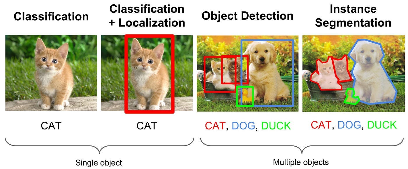
<p>Multiple object detection is the task of identifying <strong>all objects</strong> in an image by determining both <strong>what they are</strong> (classification) and <strong>where they are located</strong> (localization).</p>

<ul>
  <li><strong>Classification:</strong> Identifies what object (only one) is in the image (e.g., “CAT”).</li>
  <li><strong>Classification + Localization:</strong> Identifies what’s in the image and where it is (bounding box).</li>
  <li><strong>Multiple Object Detection:</strong> Detects <strong>multiple objects</strong> in the same scene, with bounding boxes for all of them.</li>
  <li><strong>Instance Segmentation:</strong> Extends detection by outlining the exact shapes of the objects instead of simple bounding boxes.</li>
</ul>

<h2 id="before-yolo">Before YOLO</h2>

<h3 id="deformable-parts-model">Deformable Parts Model</h3>
<hr />
<p>The Deformable Parts Model (DPM) was a pioneering object detection method that predated deep-learning approaches like R-CNN. It was introduced by <strong>Pedro Felzenszwalb et al. in 2008</strong>, and quickly became the <strong>state-of-the-art (SOTA)</strong> approach in object detection for several years.</p>

<hr />
<h3 id="how-it-works">How It Works</h3>

<ol>
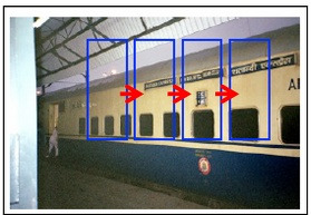
  <li><strong>Sliding Window</strong><br />
The model slides a bounding box (window) across the image at regular pixel intervals to examine different regions.</li>
</ol>
<p align="center">
  <img src="/assets/img/sliding_window.jpg" width="60%" />
</p>

<ol>
  <li><strong>Block-wise Operation</strong><br />
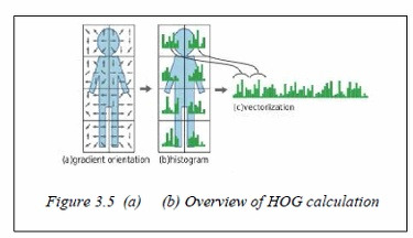
Each region is divided into small fixed-size blocks (e.g., 8×8 pixels). These blocks form the basis for feature extraction.</li>
</ol>

<p align="center">
  <img src="/assets/img/hog_feature.jpg" width="60%" />
</p>

<ol>
  <li>
    <p><strong>HOG Feature Extraction</strong><br />
For each block within a bounding box, histogram of oriented gradients (HOG) features (or similar such as SIFT) are computed. These features capture local texture and shape.</p>
  </li>
  <li>
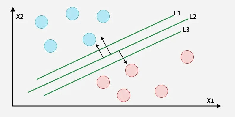
    <p><strong>Template Matching / Classification</strong><br />
Templates (or filters) pre-trained for specific object parts—such as a root filter for an entire object and part filters for subregions—are matched against the HOG features of the corresponding blocks. Each filter’s alignment produces a score (often using an SVM classifier), and the sum of these scores determines whether the object is detected.</p>
  </li>
</ol>

<p align="center">
  <img src="/assets/img/svm.png" width="75%" />
</p>

<ol>
  <li><strong>Feature Ensemble</strong><br />
The final detection decision aggregates scores from multiple templates, effectively forming an ensemble of classifiers that confirm the presence of an object in that window.</li>
</ol>

<h3 id="r-cnns">R-CNNs</h3>
<hr />
<p align="center">
  <img src="/assets/img/R_CNN_flow.png" width="90%" />
</p>

<p><strong><em>Now, did DPM remind you of something? Windows with certain sizes sliding through an image, caculating feature values along the way..</em></strong></p>

<h3 id="yes-exactly-cnns">Yes exactly! CNNs!</h3>
<p><em>*That was one of my favorite aha moments while studying object detection</em></p>

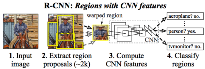
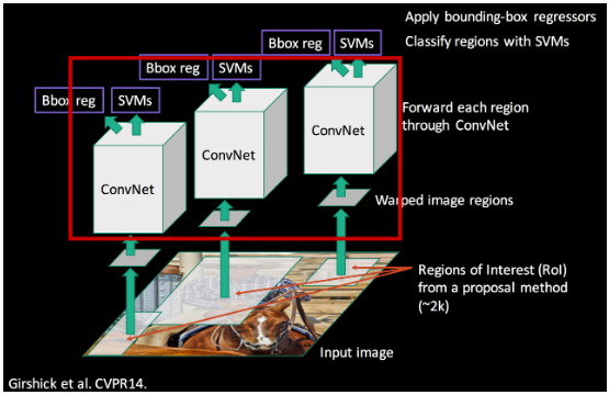
<p>It was just a matter of time untill somebody came up with the idea to use CNNs for object detection, especially after AlexNet in 2012. Evidently, Ross Girshick et al. introduced R-CNN in 2014. Using CNN for feature vector extraction, which were to fed into SVMs for classification.</p>

<hr />
<h3 id="how-it-works-1">How It Works</h3>
<p align="center">
  <img src="/assets/img/selective_search.png" width="60%" />
</p>

<ol>
  <li>
    <p><strong>Region Proposals</strong><br />
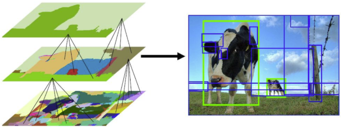
Instead of scanning the entire image with sliding windows, R-CNN first generated around 2,000 <em>region proposals</em> (candidate object locations) using algorithms like Selective Search.</p>
  </li>
  <li>
    <p><strong>Feature Extraction with CNNs</strong><br />
Each region proposal was cropped and passed through a pre-trained CNN (e.g., AlexNet) to extract features.</p>
  </li>
</ol>

<p align="center">
  <img src="/assets/img/R_CNN_flow_complete.png" width="60%" />
</p>

<ol>
  <li><strong>Classification and Refinement</strong>
    <ul>
      <li>A separate SVM classifier determined the object category for each region.</li>
      <li>A bounding-box regressor adjusted and refined the coordinates for higher accuracy.</li>
    </ul>
  </li>
</ol>

<h2 id="you-only-look-once-unified-real-time-object-detection">You Only Look Once: Unified, Real-Time Object Detection</h2>
<p align="center">
  <img src="/assets/img/yolo1.png" width="100%" />
</p>

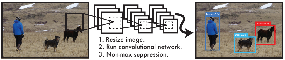
<p>YOLO, short for <em>You Only Look Once</em>, introduced a revolutionary idea: instead of treating detection as a multi-stage process, YOLO <strong>reframes object detection as a single regression problem</strong>.</p>

<ul>
  <li><strong>Input</strong>: raw image pixels (D x H x W)</li>
  <li><strong>Output</strong>: bounding box coordinates + class probabilities (S x S x (C + B*5))</li>
</ul>

<p>This means YOLO looks at the image just once (hence the name), and directly predicts <strong>what objects are present and where they are</strong>. This design eliminates the need for region proposals and repeated classification, making YOLO exceptionally fast and suitable for real-time detection.</p>

<h3 id="yolos-architecture">YOLO’s Architecture</h3>
<hr />
<p align="center">
  <img src="/assets/img/yolo_grids.png" width="90%" />
</p>

<ul>
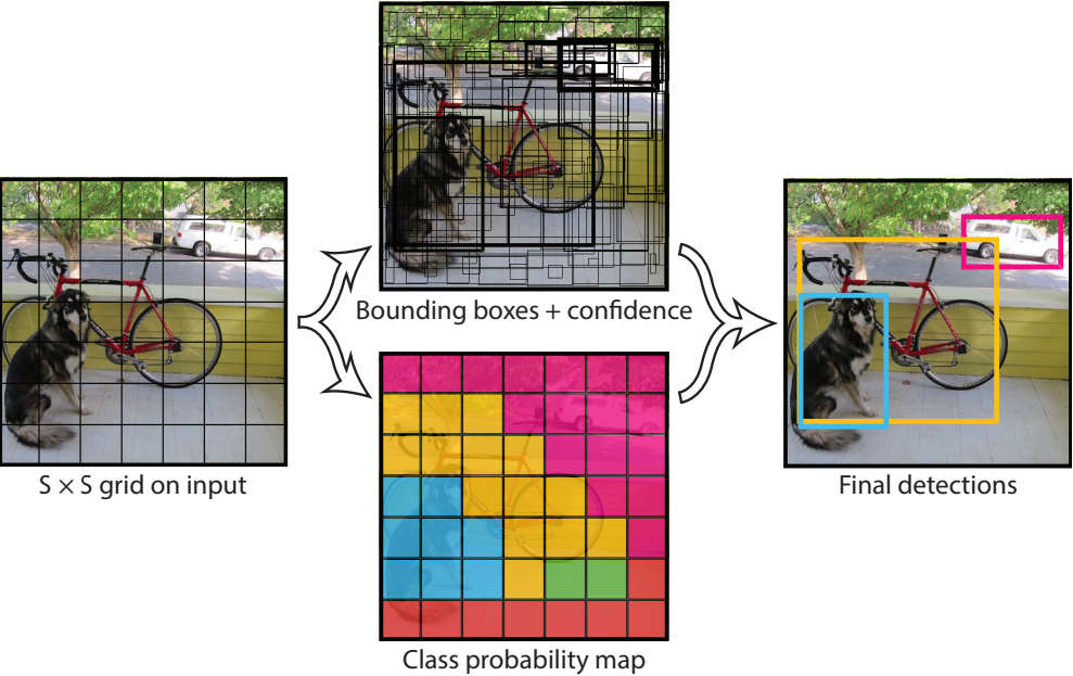
  <li>The image is divided into an <strong>S × S grid</strong>. Each grid cell predicts:
    <ul>
      <li><strong>B</strong> bounding box coordinates (x, y, width, height)</li>
      <li>A confidence score</li>
      <li><strong>C</strong> class probabilities</li>
    </ul>
  </li>
  <li>Hence, the model outputs a tensor with shape of [BATCH SIZE, C + B*5, S, S]
    <ul>
      <li>For the PASCAL VOC, C = 20</li>
      <li>and the paper states that each gird only produces 2 bound boxes, so B = 2</li>
      <li>and S = 7</li>
    </ul>
  </li>
  <li>For me personally, I’d like to interpret it backwards. Instead of thinking about splitting the <strong>input</strong> image into S x S grid, I focused more on <strong>how the ouput</strong> is S x S, and how each grid would need to have a big enough receptive field on the input image.</li>
  <li>That makes much more sense since each grid in the output should be able to <strong>see</strong> the whole image, or at least its close neighbouring grids in the input image, for the model to truly figure out the center of the object along with the width and the height of the bounding boxes.</li>
  <li>The concept of assuring a big enough receptive field on the input image for the ouput, really plays an important role here.</li>
</ul>

<p align="center">
  <img src="/assets/img/yolo_architecture.png" width="90%" />
</p>

<ul>
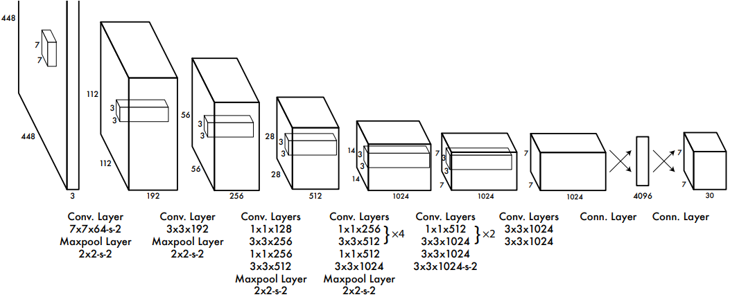
  <li>Then the network consists of <strong>24 convolutional layers</strong> (called darknet) followed by <strong>2 fully connected layers</strong>.</li>
  <li>For activations, it uses <strong>Leaky ReLU</strong> for most layers, while the final layer uses a <strong>linear activation</strong> to output bounding box coordinates.</li>
</ul>

<p>By combining these, YOLO produces dense predictions for the entire image in a single forward pass.</p>

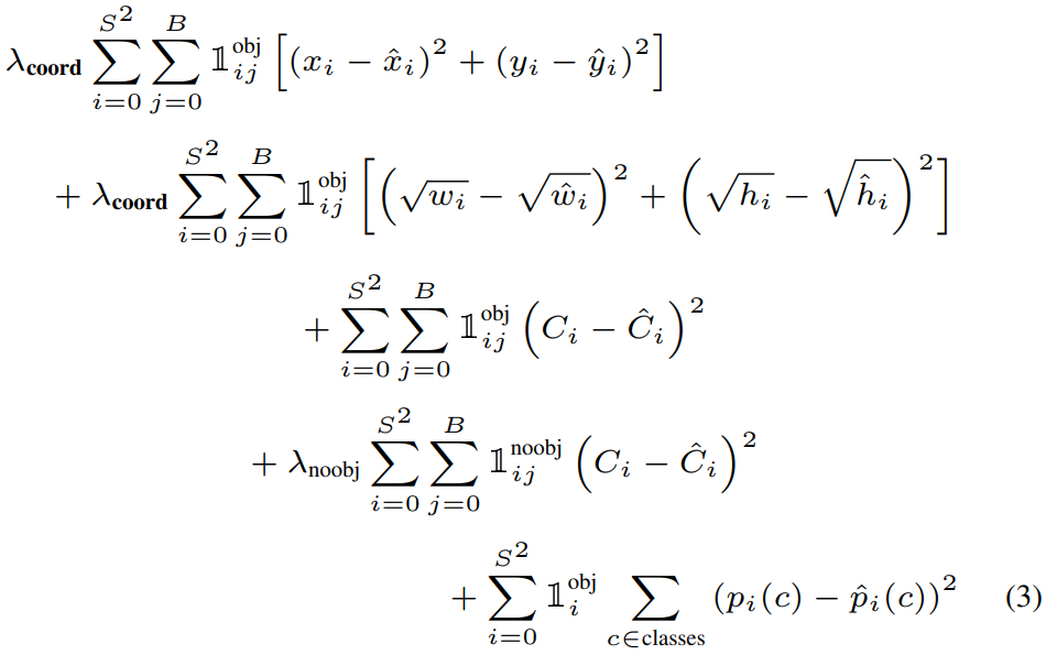
<h3 id="yolos-loss-function">YOLO’s Loss Function</h3>
<hr />

<p align="center">
  <img src="/assets/img/yolo_loss.png" width="100%" />
</p>

<p>YOLO’s loss function is a <strong>sum of multiple components</strong> that balance localization accuracy, confidence, and classification. The overall goal is to <strong>penalize wrong bounding boxes, wrong objectness scores, and wrong class predictions</strong>.</p>

<h3 id="1-localization-loss-bounding-box-coordinates">1. Localization Loss (Bounding Box Coordinates)</h3>

\[\lambda_{coord} \sum_{i=0}^{S^2} \sum_{j=0}^{B} 1_{ij}^{obj} \left[(x_i - \hat{x}_i)^2 + (y_i - \hat{y}_i)^2\right]\]

<ul>
  <li>Penalizes error in the <strong>center coordinates (x, y)</strong> of the bounding box.</li>
  <li>Only applied if the predictor is responsible for an object (<strong>$1_{ij}^{obj}=1$</strong>).</li>
  <li>Weighted by <strong>λ_coord</strong> (usually 5) to emphasize precise localization.</li>
</ul>

<h3 id="2-localization-loss-bounding-box-size">2. Localization Loss (Bounding Box Size)</h3>

\[\lambda_{coord} \sum_{i=0}^{S^2} \sum_{j=0}^{B} 1_{ij}^{obj} \left[(\sqrt{w_i} - \sqrt{\hat{w}_i})^2 + (\sqrt{h_i} - \sqrt{\hat{h}_i})^2\right]\]

<ul>
  <li>Penalizes error in the <strong>width (w)</strong> and <strong>height (h)</strong> of the bounding box.</li>
  <li>Uses <strong>square roots of w and h</strong> instead of raw values to reduce sensitivity to large boxes (so small object errors are weighted more fairly).</li>
  <li>Also weighted by <strong>λ_coord (≈5)</strong>.</li>
</ul>

<h3 id="3-confidence-loss-object-present">3. Confidence Loss (Object Present)</h3>

\[\sum_{i=0}^{S^2} \sum_{j=0}^{B} 1_{ij}^{obj} (C_i - \hat{C}_i)^2\]

<ul>
  <li>Confidence score $C_i$ represents <strong>IoU (Intersection over Union)</strong> between predicted and ground-truth box + probability of an object being present.</li>
  <li>This term penalizes error when an object <strong>is present</strong>.</li>
</ul>

<h3 id="4-confidence-loss-no-object-present">4. Confidence Loss (No Object Present)</h3>

\[\lambda_{noobj} \sum_{i=0}^{S^2} \sum_{j=0}^{B} 1_{ij}^{noobj} (C_i - \hat{C}_i)^2\]

<ul>
  <li>When no object is present in a cell (<strong>$1_{ij}^{noobj}=1$</strong>), the confidence score should ideally be 0.</li>
  <li>Penalizes false positives (predicting high confidence when there’s no object).</li>
  <li>Weighted by <strong>λ_noobj (≈0.5)</strong> to avoid overwhelming the loss, since most grid cells have no objects.</li>
</ul>

<h3 id="5-classification-loss">5. Classification Loss</h3>

\[\sum_{i=0}^{S^2} 1_i^{obj} \sum_{c \in classes} (p_i(c) - \hat{p}_i(c))^2\]

<ul>
  <li>Applied only to cells containing an object.</li>
  <li>Penalizes error between predicted class probabilities $p_i(c)$ and true labels $\hat{p}_i(c)$.</li>
  <li>Uses sum-squared error for all classes.</li>
</ul>

<hr />

<h3 id="the-role-of-λ-lambdas">The Role of λ (Lambdas)</h3>
<ul>
  <li><strong>λ_coord (5):</strong> Increases weight of localization error (bounding box coordinates + size). Without this, classification and confidence terms would dominate.</li>
  <li><strong>λ_noobj (0.5):</strong> Decreases weight for background confidence error, since most cells have no objects and would otherwise overwhelm the loss.</li>
</ul>

<h2 id="advance-in-research">Advance in Research?</h2>

<p align="center">
  <img src="/assets/img/yolov9.png" width="100%" />
</p>

<ul>
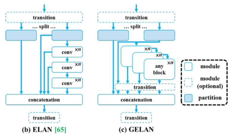
  <li><strong>YOLO v9 – Learning What You Want to Learn Using Programmable Gradient Information (2024)</strong><br />
Introduces <strong>Programmable Gradient Information (PGI)</strong> to improve training signals and the <strong>Generalized Efficient Layer Aggregation Network (GELAN)</strong> (a generalization of ELAN) for efficient architecture design.</li>
</ul>

<p align="center">
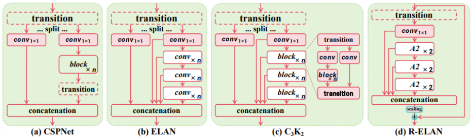
  <img src="/assets/img/yolo_attention.png" width="100%" />
</p>

<ul>
  <li><strong>YOLO v12 – Attention-Centric Object Detection (2025)</strong><br />
Proposes an <strong>attention-centric</strong> YOLO that keeps real-time speed. Key components are the <strong>Area Attention module (A2)</strong> and <strong>Residual Efficient Layer Aggregation Networks (R-ELAN)</strong></li>
</ul>

<h2 id="implementing-with-pytorch">Implementing with PyTorch</h2>
<p>The architecture is basically in the paper, and so is the loss. It is relatively straightforward and easy to code. So you can check it out in my GitHub repo.</p>
<ul>
  <li><a href="https://github.com/kmsrogerkim/AI-Models-Collection">https://github.com/kmsrogerkim/AI-Models-Collection</a></li>
</ul>

<p>And I would have to give credit to <a href="https://github.com/aladdinpersson">Aladdin Persson</a> for implementing the model and everything else prior to me.</p>
<ul>
  <li><a href="https://github.com/aladdinpersson/Machine-Learning-Collection/tree/master/ML/Pytorch/object_detection/YOLO">https://github.com/aladdinpersson/Machine-Learning-Collection/tree/master/ML/Pytorch/object_detection/YOLO</a></li>
</ul>

<h2 id="references">References</h2>

<ul>
  <li>
    <p>Redmon, J., Divvala, S., Girshick, R., &amp; Farhadi, A. (2016). <em>You only look once: Unified, real-time object detection</em>. In <em>Proceedings of the IEEE Conference on Computer Vision and Pattern Recognition (CVPR)</em> (pp. 779–788).</p>
  </li>
  <li>
    <p>Wang, C.-Y., Yeh, I.-H., &amp; Liao, H.-Y. M. (2024). <em>YOLOv9: Learning what you want to learn using programmable gradient information</em>. In <em>European Conference on Computer Vision (ECCV)</em>. Cham: Springer Nature Switzerland.</p>
  </li>
  <li>
    <p>Tian, Y., Ye, Q., &amp; Doermann, D. (2025). <em>YOLOv12: Attention-centric real-time object detectors</em>. <em>arXiv preprint</em> arXiv:2502.12524.</p>
  </li>
  <li>
    <p>Augmented Startups. (2023). <em>Object detection vs classification in computer vision</em>. <em>Medium</em>. Retrieved from <a href="https://augmentedstartups.medium.com/object-detection-vs-classification-in-computer-vision-123c437e33be">https://augmentedstartups.medium.com/object-detection-vs-classification-in-computer-vision-123c437e33be</a></p>
  </li>
  <li>
    <p>89douner. (2020). <em>[Deformable Parts Model Explanation]</em>. <em>Tistory Blog</em>. Retrieved from <a href="https://89douner.tistory.com/82">https://89douner.tistory.com/82</a></p>
  </li>
  <li>
    <p>Ganghee Lee. (2020). <em>[R-CNN Object Detection Explanation]</em>. <em>Tistory Blog</em>. Retrieved from <a href="https://ganghee-lee.tistory.com/35">https://ganghee-lee.tistory.com/35</a></p>
    <h2 id="written-by">Written by</h2>
    <blockquote>
      <p><strong>Roger Kim</strong><br />
<a href="https://github.com/kmsrogerkim"><img src="https://img.shields.io/badge/GitHub-181717?logo=github&amp;logoColor=white" alt="GitHub" /></a> <a href="https://www.linkedin.com/in/kmsrogerkim/"><img src="https://img.shields.io/badge/LinkedIn-0A66C2?logo=linkedin&amp;logoColor=white" alt="LinkedIn" /></a></p>
    </blockquote>
  </li>
</ul>]]></content><author><name>Roger Kim</name></author><category term="AI" /><category term="AI" /><category term="CV" /><summary type="html"><![CDATA[Evolution of Multiple Object Detection and the Rise of YOLO Object detection is the action of detecting what objects are in an image, and pinpointng where each object is located. This task lies at the core of many real-world applications such as autonomous driving, medical imaging, video surveillance, and more.]]></summary></entry><entry><title type="html">Understanding Denoising Diffusion Probabilistic Models</title><link href="https://kmsrogerkim.github.io/ai/ddpm/" rel="alternate" type="text/html" title="Understanding Denoising Diffusion Probabilistic Models" /><published>2025-04-01T00:00:00+00:00</published><updated>2025-04-01T00:00:00+00:00</updated><id>https://kmsrogerkim.github.io/ai/ddpm</id><content type="html" xml:base="https://kmsrogerkim.github.io/ai/ddpm/"><![CDATA[<h2 id="introduction">Introduction</h2>
<p>As a part of a group study session at my college’s artificial intelligence club <a href="https://github.com/HanyangTechAI">HYU HAI</a>, I came across the <em>Denoising Diffusion Probabilistic Models</em> paper. We studied the paper together, and here’s what I learned from it.</p>

<p><strong>Citation</strong></p>

<p>[1] J. Ho, A. Jain, and P. Abbeel, “Denoising Diffusion Probabilistic Models,” <em>arXiv:2006.11239 [cs, stat]</em>, Dec. 2020, Available: <a href="https://arxiv.org/abs/2006.11239">https://arxiv.org/abs/2006.11239</a></p>

<p>[2] Kingma, Diederik P., and Max Welling. “Auto-encoding variational bayes.” 20 Dec. 2013, Available:  <a href="https://arxiv.org/abs/1312.6114">https://arxiv.org/abs/1312.6114</a></p>

<p>[3] MyeonGu Jo’s GitHub repository Available: <a href="https://github.com/MyeongGuJo?tab=repositories">https://github.com/MyeongGuJo?tab=repositories</a></p>

<p><img src="/assets/img/ddpm.png" alt="" /></p>

<h2 id="forward-process">Forward Process</h2>
<p><strong>Forward process is the process of adding noise to an image</strong>. It is also called diffusion process. Let the original image be represented by $X_0$. The forward process is defined as</p>

\[q(X_{1:T}|X_0) := \prod_{t=1}^{T} q(X_t|X_{t-1})\]

\[q(X_t|X_{t-1}) := \mathcal{N}(X_t; \sqrt{1 - \beta_t} X_{t-1}, \beta_t I)\]

<p>According to this definition, the calculation needs to be done $T$ times in order to reach the final state, $X_T$, forming a <strong>Markov chain</strong>. This can be computationally expansive. In order to solve this problem, the paper cites <em>Auto-encoding variational Bayes</em> paper <a href="https://arxiv.org/abs/1312.6114">[2]</a>, and reparameterizes the diffusion process into</p>

\[q(X_t | X_0) = \mathcal{N}(X_t; \sqrt{\bar{\alpha}_t} X_0, (1 - \bar{\alpha}_t) I)\]

<p>where</p>
<div align="center">
  <img src="/assets/img/ddpm_alpha_and_alpha_hat.png" alt="DDPM Algorithm 1 and 2" width="60%" />
</div>

<p>Notice how <strong>the diffusion process is now defined as a single gaussian distribution</strong>, with a new parameter $\alpha$. This reparameterization allow us to <strong>skip the markov chain</strong> and directly reach the image with noise at step $t$, $X_t$.</p>

<p>Now, the paper further reparameterizes them in terms of $\tilde{\mu}_t$ and $\tilde{\beta}_t$. These parameters will later be used for direct comparison between the reverse process’s values in the loss function. Now the forward process takes the final form of</p>

\[q(X_t | X_0) = \mathcal{N}(X_t; \tilde{\mu}_t (X_t, X_0), \tilde{\beta}_t I)\]

\[\tilde{\mu}_t(X_t, X_0) := \frac{\sqrt{\bar{\alpha}_t - 1} \beta_t}{1 - \bar{\alpha}_t} X_0 + \frac{\sqrt{\alpha_t (1 - \bar{\alpha}_{t-1})}}{1 - \bar{\alpha}_t} X_t\]

\[\quad \tilde{\beta}_t := \frac{1 - \bar{\alpha}_{t-1}}{1 - \bar{\alpha}_t} \beta_t\]

<p>These reparametrizations gave me headahces; but here’s how I understand it. ~μt
is basically the answer for the diffusion process’s posterior’s expacted value. It is the value that we are aiming to predict using our neural network. ~Bt represents the variability of the noise in the diffusion process, influencing <em>how much</em> the original data gets altered.</p>

<h2 id="reverse-process">Reverse Process</h2>
<p>Now, the goal of this paper is to denoise that $X_T$ image back into $X_0$. In order to do that, a reverse process is defined as follow.</p>

\[p_\theta(X_{0:T}) := p(X_T) \prod_{t=1}^{T} p_\theta(X_{t-1}|X_t)\]

\[p_\theta(X_{t-1}|X_t) := \mathcal{N}(X_{t-1}; \mu_\theta(X_t, t),\sum_\theta(X_t, t))\]

<p>Notice how there is a little $\theta$ under the $p$ function, $\mu$ function and the $\sum$ function? That represents that the value of those functions can be altered by the parameters, which will be calculated by neural network.</p>

<h2 id="loss-function">Loss Function</h2>
<p>Now, in order to train our neural network to get $\tilde{\mu}_t$, we need to define loss function. The loss function used here is defiend based on the variational bound on negative log likelihood.</p>

<p>Given a negative log likelihood $\mathbb{E} [-\log p_\theta(X_0)]$, the paper takes variational bound on that likelihood via the following equation and defines the Loss function $L$</p>

\[\mathbb{E}[-\log p_{\theta}(X_0)]\]

\[\leq \mathbb{E}_q[-\log \frac{p_{\theta}(X_{0:T})}{q(X_{1:T}|X_0)}]\]

\[= \mathbb{E}_q[-\log p(X_T) - \sum_{t\geq1} \log \frac{p_{\theta}(X_{t-1}|X_t)}{q(X_t|X_{t-1})}] =: L\]

<p>To represent the mean $\mu_\theta(X_t, t)$, the paper proposes a specific parameterization motivated by the following analysis of $L_t$. With first setting the variance for the reverse process as $\sigma^2_t I$ we can write:</p>

\[L_{t-1} = \mathbb{E}_{q} \left[ \frac{1}{2 \sigma_{t}^{2}} \| \tilde{\mu}_{t}(x_{t}, x_{0}) - \mu_{0}(x_{t}, t) \|^{2} \right] + C\]

<p>Then, we can just simply rewrite it in terms of $\epsilon$, the guassian noise added to the image
\(L_{t-1} = \mathbb{E}_{x_0, \epsilon} \left[ \frac{1}{2 \sigma_t^2} \left\| \frac{1}{\sqrt{\alpha_t}} \left( x_t(x_0, \epsilon) - \frac{\beta_t}{\sqrt{1 - \alpha_t}} \epsilon \right) - \mu_0(x_t(x_0, \epsilon), t) \right\|^2 \right]\)</p>

<p>Notice how the expacted value is now represented by $X_0$ and $\epsilon$, $\alpha$ and $\mu_\theta$. The expacted value is also continuosly simplified later in the paper, but I am just going to mention the simple loss function (equation (14)).</p>

\[L_{\text{simple}}(\theta) := \mathbb{E}_{t, x_0, \epsilon} \left[ \left\| \epsilon - \epsilon_\theta \left( \sqrt{\bar{\alpha}_t} x_0 + \sqrt{1 - \bar{\alpha}_t} \epsilon, t \right) \right\|^2 \right]\]

<h2 id="summerizing-the-mathematical-concepts">Summerizing the mathematical concepts</h2>
<p>“To summarize, we can train the reverse process mean function approximator $\mu_\theta$ to predict $\tilde{\mu}_\theta$, or by modifying its parameterization, we can train it to predict $\epsilon$” [1].</p>

<p>That is just basically what we are trying to do, and why the paper reparametrized the functions.</p>

<h2 id="algorithms">Algorithms</h2>
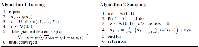
<div align="center">
  <img src="/assets/img/ddpm_algorithm_1_2.png" alt="DDPM Algorithm 1 and 2" />
</div>

<div align="center">
  <img src="/assets/img/ddpm_algorithm_3_4.png" alt="DDPM Algorithm 3 and 4" />
</div>

<p><strong>Algorithm 1</strong> is the process of training the neural networking using the loss function defined above (with $\epsilon$). You can see how we take gradient descent step to train our neural network so that the $\hat{\mu_t}$ gets close to $\mu_\theta$.</p>

<p><strong>Algorithm 2</strong> is the process of calculating $X_0$ from $X_T$ using our reverse function and the parameters.</p>

<p><strong>Algorithm 3</strong> and <strong>Algorithm 4</strong> is the sender and the receiver for the image. The sender encodes the image using $X_t$ ~ q(X_T|X_0).
The receiver decodes the image using revers process function.</p>

<h2 id="the-neural-network">The Neural Network</h2>
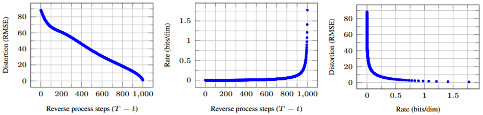
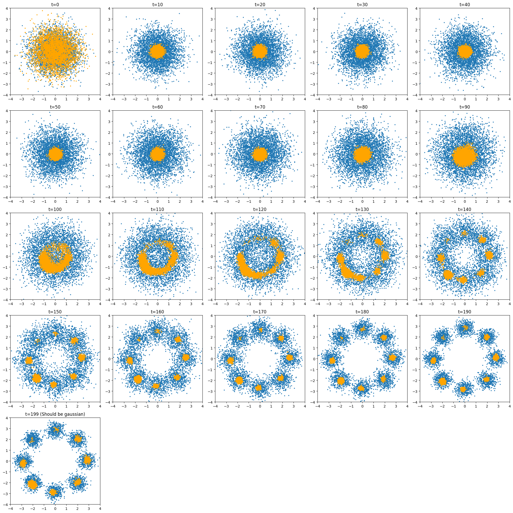
<p>The paper shares the result of its training using neural network. The evaluation using RSME is like the image below. The paper used <strong>U-Net</strong> backbone neural network. <em>“To represent the reverse process, we use a U-Net backbone similar to an unmasked PixelCNN++”</em> [1].
<img src="/assets/img/ddpm_rsme.png" alt="" />
From J. Ho., et al., DDPM, 2020, Figure 5: Unconditional CIFAR10 test set rate-distortion vs. time. Distortion is measured in root mean squared error on a [0, 255] scale. See Table 4 for details.</p>
<h2 id="code-implementation">Code Implementation</h2>
<p><img src="/assets/img/mgj_ddpm_hayaku.png" alt="" />
The person who taught me all this, <a href="https://github.com/MyeongGuJo">MyeonGu Jo</a> from Hanyang University, has a simple walk-through google colab file that implements this paper. In <a href="https://github.com/MyeongGuJo/hayaku-250322">this specific repository</a> he used Multi-Layer Perceptron for a basic demonstration. You can visit the repository here</p>
<ul>
  <li><a href="https://github.com/MyeongGuJo/hayaku-250322">https://github.com/MyeongGuJo/hayaku-250322</a></li>
</ul>

<p>Click on the <a href="https://colab.research.google.com/github/MyeongGuJo/hayaku-250322/blob/main/hayaku_diffusion.ipynb#scrollTo=AIXGa_RfQaq-">Open in Colab</a> button to run it yourself.</p>

<p>Or checkout his U-Net implementation here</p>
<ul>
  <li><a href="https://github.com/MyeongGuJo/diffusion/tree/main">https://github.com/MyeongGuJo/diffusion/tree/main</a></li>
</ul>

<h2 id="written-by">Written by</h2>
<blockquote>
  <p><strong>Roger Kim</strong><br />
<a href="https://github.com/kmsrogerkim"><img src="https://img.shields.io/badge/GitHub-181717?logo=github&amp;logoColor=white" alt="GitHub" /></a> <a href="https://www.linkedin.com/in/kmsrogerkim/"><img src="https://img.shields.io/badge/LinkedIn-0A66C2?logo=linkedin&amp;logoColor=white" alt="LinkedIn" /></a></p>
</blockquote>]]></content><author><name>Roger Kim</name></author><category term="AI" /><category term="AI" /><category term="Diffusion" /><category term="CV" /><summary type="html"><![CDATA[Introduction As a part of a group study session at my college’s artificial intelligence club HYU HAI, I came across the Denoising Diffusion Probabilistic Models paper. We studied the paper together, and here’s what I learned from it.]]></summary></entry><entry><title type="html">Github Actions to Automate Image pushing &amp;amp; Django Testing</title><link href="https://kmsrogerkim.github.io/devops/github-actions/" rel="alternate" type="text/html" title="Github Actions to Automate Image pushing &amp;amp; Django Testing" /><published>2024-11-26T00:00:00+00:00</published><updated>2024-11-26T00:00:00+00:00</updated><id>https://kmsrogerkim.github.io/devops/github-actions</id><content type="html" xml:base="https://kmsrogerkim.github.io/devops/github-actions/"><![CDATA[<h2 id="introduction">Introduction</h2>
<p>In this post, I would like to discuss how I set up a CI/CD pipline for my <a href="https://toyki-homepage.vercel.app/">toyki</a>project. I automated unit testing for my backend application built with Django, and the process of creating a docker image of it and pushing it to AWS ECR, all using GitHub actions.</p>

<h2 id="getting-started">Getting Started</h2>
<p>To set up a GitHub Actions workflow, go to the <code class="language-plaintext highlighter-rouge">Actions</code> tab in your repository and click <code class="language-plaintext highlighter-rouge">New Workflow</code>. Choose a template, configure the .yml file, and commit it. This automatically creates a <code class="language-plaintext highlighter-rouge">.github/workflows/</code> directory containing the .yml files, which define your workflows.</p>

<p>Alternatively, you can manually create the <code class="language-plaintext highlighter-rouge">.github/workflows/</code> directory and add .yml files yourself, and GitHub will recognize and run them.</p>

<p>Here’s how the beginning of the .yml files would look like. As you can see below, you can configure when your workflows will run. The .yml below shows that the name of the workflow is <code class="language-plaintext highlighter-rouge">Django CI</code> and it will run when</p>

<ol>
  <li>a commit is pushed to the <code class="language-plaintext highlighter-rouge">main</code> or the <code class="language-plaintext highlighter-rouge">development</code> branch</li>
  <li>when a pull request is created on them.</li>
</ol>

<div class="language-yml highlighter-rouge"><div class="highlight"><pre class="highlight"><code><span class="na">name</span><span class="pi">:</span> <span class="s">Django CI</span>

<span class="na">on</span><span class="pi">:</span>
  <span class="na">push</span><span class="pi">:</span>
    <span class="na">branches</span><span class="pi">:</span> <span class="pi">[</span> <span class="s2">"</span><span class="s">main"</span><span class="pi">,</span> <span class="s2">"</span><span class="s">development"</span> <span class="pi">]</span>
  <span class="na">pull_request</span><span class="pi">:</span>
    <span class="na">branches</span><span class="pi">:</span> <span class="pi">[</span> <span class="s2">"</span><span class="s">main"</span><span class="pi">,</span> <span class="s2">"</span><span class="s">development"</span> <span class="pi">]</span>
</code></pre></div></div>

<h2 id="automate-unit-tests">Automate Unit Tests</h2>
<p>So first, I created unit tests for my REST API, using pytest. Then I created a .yml file in the <code class="language-plaintext highlighter-rouge">.github/workflows/</code> directory which looks something like this.</p>

<div class="language-yml highlighter-rouge"><div class="highlight"><pre class="highlight"><code><span class="na">name</span><span class="pi">:</span> <span class="s">Django CI</span>

<span class="na">on</span><span class="pi">:</span>
  <span class="na">push</span><span class="pi">:</span>
    <span class="na">branches</span><span class="pi">:</span> <span class="pi">[</span> <span class="s2">"</span><span class="s">main"</span><span class="pi">,</span> <span class="s2">"</span><span class="s">development"</span> <span class="pi">]</span>
  <span class="na">pull_request</span><span class="pi">:</span>
    <span class="na">branches</span><span class="pi">:</span> <span class="pi">[</span> <span class="s2">"</span><span class="s">main"</span><span class="pi">,</span> <span class="s2">"</span><span class="s">development"</span> <span class="pi">]</span>

<span class="na">jobs</span><span class="pi">:</span>
  <span class="na">test</span><span class="pi">:</span>
    <span class="na">runs-on</span><span class="pi">:</span> <span class="s">ubuntu-latest</span>

    <span class="na">services</span><span class="pi">:</span>
      <span class="na">postgres</span><span class="pi">:</span>
        <span class="na">image</span><span class="pi">:</span> <span class="s">postgres:14-alpine</span>
        <span class="na">env</span><span class="pi">:</span>
        <span class="c1"># necessary env variables to set up your postgreSQL db</span>
        <span class="na">ports</span><span class="pi">:</span>
          <span class="pi">-</span> <span class="s">5432:5432</span>
      <span class="na">memcached</span><span class="pi">:</span>
        <span class="na">image</span><span class="pi">:</span> <span class="s">memcached:1.6.14-alpine</span>
        <span class="na">ports</span><span class="pi">:</span>
          <span class="pi">-</span> <span class="s">11211:11211</span>

    <span class="na">strategy</span><span class="pi">:</span>
      <span class="na">max-parallel</span><span class="pi">:</span> <span class="m">4</span>
      <span class="na">matrix</span><span class="pi">:</span>
        <span class="na">python-version</span><span class="pi">:</span> <span class="pi">[</span><span class="s1">'</span><span class="s">3.10'</span><span class="pi">]</span>

    <span class="na">steps</span><span class="pi">:</span>
      <span class="pi">-</span> <span class="na">uses</span><span class="pi">:</span> <span class="s">actions/checkout@v4</span>

      <span class="pi">-</span> <span class="na">name</span><span class="pi">:</span> <span class="s">Set up Python $</span>
        <span class="na">uses</span><span class="pi">:</span> <span class="s">actions/setup-python@v3</span>
        <span class="na">with</span><span class="pi">:</span>
          <span class="na">python-version</span><span class="pi">:</span> <span class="s">$</span>

      <span class="pi">-</span> <span class="na">name</span><span class="pi">:</span> <span class="s">Install Dependencies</span>
        <span class="na">run</span><span class="pi">:</span> <span class="pi">|</span>
          <span class="s">python -m pip install --upgrade pip</span>
          <span class="s">pip install poetry</span>
          <span class="s">poetry install</span>

      <span class="pi">-</span> <span class="na">name</span><span class="pi">:</span> <span class="s">Generate Environment Variables File</span>
        <span class="na">run</span><span class="pi">:</span> <span class="pi">|</span>
          <span class="s">echo "DJANGO_SECRET_KEY=$DJANGO_SECRET_KEY" &gt;&gt; .env.dev</span>
        <span class="c1"># other sensitive env variables that are stored in Github secrets</span>

        <span class="na">env</span><span class="pi">:</span>
          <span class="na">DJANGO_SECRET_KEY</span><span class="pi">:</span> <span class="s">$</span>
          <span class="na">API_KEY</span><span class="pi">:</span> <span class="s">$</span>
          <span class="c1"># declare your env variables here</span>
          <span class="c1"># so that the system can reach them on the command above with the $ sign</span>

      <span class="pi">-</span> <span class="na">name</span><span class="pi">:</span> <span class="s">Run Tests</span>
        <span class="na">run</span><span class="pi">:</span> <span class="pi">|</span>
          <span class="s">poetry run pytest &lt;your directory to the test code file&gt;</span>
        <span class="c1"># e.x: tests/test_django.py</span>

        <span class="na">env</span><span class="pi">:</span>
          <span class="na">ENVIRONMENT</span><span class="pi">:</span> <span class="s1">'</span><span class="s">development'</span>
          <span class="c1"># other env variables that are not sensitive and</span>
          <span class="c1"># can directly be stored as text in .yml file</span>
</code></pre></div></div>

<ul>
  <li><code class="language-plaintext highlighter-rouge">services</code>
    <ul>
      <li>These services can be used for the steps that follow; in this case unit testing.</li>
    </ul>
  </li>
  <li><code class="language-plaintext highlighter-rouge">strategy</code>
    <ul>
      <li><code class="language-plaintext highlighter-rouge">max-parallel</code>: this configures how many runs can run simultaneously (parallel)</li>
      <li><code class="language-plaintext highlighter-rouge">matrix</code>: sets up some variables that can be used through out the run</li>
    </ul>
  </li>
  <li><code class="language-plaintext highlighter-rouge">steps</code>
    <ul>
      <li>This sections basically states what the github actions will do. It is very similar to how Dockerfile works if you think about it. You just tell the container to run certain commads.</li>
      <li>The only thing that you might not be familiar with would be the <code class="language-plaintext highlighter-rouge">uses</code> command used along with <code class="language-plaintext highlighter-rouge">actions/checkout$v4</code> and <code class="language-plaintext highlighter-rouge">actions/setup-python@v3</code></li>
    </ul>
  </li>
  <li><code class="language-plaintext highlighter-rouge">secrets</code>
    <ul>
      <li>The secret env variables can be set in <code class="language-plaintext highlighter-rouge">github.com/your_id/your_repo/settings/secrets/actions</code>path.</li>
      <li>And they can be reacehd by doing <code class="language-plaintext highlighter-rouge">$</code> as can see from above.</li>
    </ul>
  </li>
  <li><code class="language-plaintext highlighter-rouge">uses</code>
    <ul>
      <li>This keyword specifies an action to be executed as part of the workflow. Actions, just like the one we are creating right now, are pre-built, reusable units of code that perform specific tasks.</li>
      <li><code class="language-plaintext highlighter-rouge">actions/checkout@v4</code>: an actions maintained by GitHub that checks out the code from the repository to whatever the envrionment the actions will be ran (upload it to VM).</li>
      <li><code class="language-plaintext highlighter-rouge">actions/setup-python@v3</code>: It sets up a Python environment in the runner. It ensures that the specified version of Python is installed and available in the <code class="language-plaintext highlighter-rouge">PATH</code>, which, if you have ever tried setting up Python on different machines, can sometimes be a huge pain in the ass.</li>
    </ul>
  </li>
</ul>

<h2 id="automate-image-pushing-to-aws-ecr">Automate Image Pushing to AWS ECR</h2>
<p>If you click on the <code class="language-plaintext highlighter-rouge">New Workflow</code> button in the actions tab, you can see <code class="language-plaintext highlighter-rouge">Deploy to Amazon ECS</code>. This action already includes image creation and pushing to ECR. So I just used that. Here’s how it looks like.</p>

<div class="language-yml highlighter-rouge"><div class="highlight"><pre class="highlight"><code><span class="na">name</span><span class="pi">:</span> <span class="s">Push Image to ECR</span>

<span class="na">on</span><span class="pi">:</span>
  <span class="na">push</span><span class="pi">:</span>
    <span class="na">branches</span><span class="pi">:</span> <span class="pi">[</span> <span class="s2">"</span><span class="s">main"</span> <span class="pi">]</span>

<span class="na">env</span><span class="pi">:</span>
  <span class="na">AWS_REGION</span><span class="pi">:</span> <span class="s">your_region_here</span>
  <span class="na">ECR_REPOSITORY</span><span class="pi">:</span> <span class="s">your_ecr_name_here</span>
  <span class="c1"># e.x: toyki</span>

<span class="na">permissions</span><span class="pi">:</span>
  <span class="na">contents</span><span class="pi">:</span> <span class="s">read</span>

<span class="na">jobs</span><span class="pi">:</span>
  <span class="na">push_image</span><span class="pi">:</span>
    <span class="na">name</span><span class="pi">:</span> <span class="s">push-image</span>
    <span class="na">runs-on</span><span class="pi">:</span> <span class="s">ubuntu-latest</span>
    <span class="na">environment</span><span class="pi">:</span> <span class="s">production</span>
    <span class="c1"># set the env variable of `envronment` to production</span>
    <span class="c1"># since some of my codes runs differently depending on this</span>
    <span class="c1"># env variable</span>

    <span class="na">steps</span><span class="pi">:</span>
    <span class="pi">-</span> <span class="na">name</span><span class="pi">:</span> <span class="s">Checkout</span>
      <span class="na">uses</span><span class="pi">:</span> <span class="s">actions/checkout@v4</span>

    <span class="pi">-</span> <span class="na">name</span><span class="pi">:</span> <span class="s">Configure AWS credentials</span>
      <span class="na">uses</span><span class="pi">:</span> <span class="s">aws-actions/configure-aws-credentials@v1</span>
      <span class="na">with</span><span class="pi">:</span>
        <span class="na">aws-access-key-id</span><span class="pi">:</span> <span class="s">$</span>
        <span class="na">aws-secret-access-key</span><span class="pi">:</span> <span class="s">$</span>
        <span class="na">aws-region</span><span class="pi">:</span> <span class="s">$</span>

    <span class="pi">-</span> <span class="na">name</span><span class="pi">:</span> <span class="s">Login to Amazon ECR</span>
      <span class="na">id</span><span class="pi">:</span> <span class="s">login-ecr</span>
      <span class="na">uses</span><span class="pi">:</span> <span class="s">aws-actions/amazon-ecr-login@v1</span>

    <span class="pi">-</span> <span class="na">name</span><span class="pi">:</span> <span class="s">Build, tag, and push image to Amazon ECR</span>
      <span class="na">id</span><span class="pi">:</span> <span class="s">build-image</span>
      <span class="na">env</span><span class="pi">:</span>
        <span class="na">ECR_REGISTRY</span><span class="pi">:</span> <span class="s">$</span>
      <span class="na">run</span><span class="pi">:</span> <span class="pi">|</span>
        <span class="s">DJANGO_IMAGE_TAG=$(cat django_image_tag.txt)</span>
      <span class="c1"># I specify the image tag for my production images in a text file</span>
      <span class="c1"># in the repository. It is updated everytime a PR is merged to main</span>

        <span class="s">docker build -t $ECR_REGISTRY/$ECR_REPOSITORY:$DJANGO_IMAGE_TAG .</span>
        <span class="s">docker push $ECR_REGISTRY/$ECR_REPOSITORY:$DJANGO_IMAGE_TAG</span>
        <span class="s">echo "image=$ECR_REGISTRY/$ECR_REPOSITORY:$DJANGO_IMAGE_TAG" &gt;&gt; $GITHUB_OUTPUT</span>
</code></pre></div></div>
<p>There is nothing special here. There are a lot of pre-built actions from aws themselves that you can use in your GitHub actions. For example, the <code class="language-plaintext highlighter-rouge">aws-actions/configure-aws-credentials</code> and <code class="language-plaintext highlighter-rouge">aws-actions/amazon-ecr-login@v1</code> actions are used in this action.</p>

<h2 id="conclusion">Conclusion</h2>
<p>While doing this, I felt like everything is just a bash script at its core. GitHub sets up an isolated environment for you either using VM (default) or containers. Then you tell the machine to run some commands. Just like Dockerfile, and just like a bash script.</p>

<p>In fact, I am currently doing another project with the HYU’s Vibro Acoustics lab, where I have to manually set up Docker and everything in an EC2 instance. In the process, I made up a bash scrip of my own that automates a lot of the set up process. I also created a bash script that pulls image from ECR and set up some variables and run the image as container. While I was doing that, I thought to myself that maybe this is just what is happening behind the scene for AWS’s ECS service at its core.</p>

<p>Anyways, I hope my post helped make your developing life better.</p>

<h2 id="written-by">Written by</h2>
<blockquote>
  <p><strong>Roger Kim</strong><br />
<a href="https://github.com/kmsrogerkim"><img src="https://img.shields.io/badge/GitHub-181717?logo=github&amp;logoColor=white" alt="GitHub" /></a> <a href="https://www.linkedin.com/in/kmsrogerkim/"><img src="https://img.shields.io/badge/LinkedIn-0A66C2?logo=linkedin&amp;logoColor=white" alt="LinkedIn" /></a></p>
</blockquote>]]></content><author><name>Roger Kim</name></author><category term="devops" /><category term="django" /><category term="docker" /><category term="aws" /><category term="devops" /><category term="ci/cd" /><category term="github actions" /><summary type="html"><![CDATA[Introduction In this post, I would like to discuss how I set up a CI/CD pipline for my toykiproject. I automated unit testing for my backend application built with Django, and the process of creating a docker image of it and pushing it to AWS ECR, all using GitHub actions.]]></summary></entry><entry><title type="html">Customize DRF Simplejwt</title><link href="https://kmsrogerkim.github.io/django/customize-opensource/" rel="alternate" type="text/html" title="Customize DRF Simplejwt" /><published>2024-11-18T00:00:00+00:00</published><updated>2024-11-18T00:00:00+00:00</updated><id>https://kmsrogerkim.github.io/django/customize-opensource</id><content type="html" xml:base="https://kmsrogerkim.github.io/django/customize-opensource/"><![CDATA[<h2 id="introduction">Introduction</h2>
<p>In this post, I am going to talk about how I customized a part of the <a href="https://github.com/jazzband/djangorestframework-simplejwt">drf-simplejwt repository</a> to build a custom authentification flow for my <a href="https://toyki-homepage.vercel.app/">toyki project</a>. It is a <strong>very simple</strong> customization. There was a specific need for a custom workflow with jwt tokens from front-end, which I will talk about in detail later.</p>

<h2 id="background">Background</h2>
<p>The project required a custom workflow to determine whether a pair of refresh and access token were valid or not. Client would pass the tokens all together to the <code class="language-plaintext highlighter-rouge">api/token/valid</code> endpoint. Then the server would have to determince if the access and the refresh token are valid or not. The problem was that when the access token was passed through the header directly, without the bearer prefix, CORS error would occur. However, when the access token is passed through the header <strong><em>with</em></strong> the bearer header, the default JWTAuthentication method provided by the simplejwt would immediately return 401 when the access token is invalid, regardless of the validity of the refresh token, and the permission class of the view. So I decided to set up a simple custom authentication class based on the JWTAuthentication class in the simplejwt, that checks for both the access and refresh tokens’ validity.</p>

<h2 id="original-code">Original Code</h2>
<p>First of all, I searched for the code for JWTAuthentication from the simplejwt repo. If you check the DEFAULT_AUTHENTICATION_CLASSES tuple in <code class="language-plaintext highlighter-rouge">settings.py</code> it is probably set to the JWTAuthentication class, which, if you recall, was configured by you when you added the simplejwt to your service.</p>
<div class="language-python highlighter-rouge"><div class="highlight"><pre class="highlight"><code><span class="n">REST_FRAMEWORK</span> <span class="o">=</span> <span class="p">{</span>
    <span class="s">'DEFAULT_AUTHENTICATION_CLASSES'</span><span class="p">:</span> <span class="p">(</span>
        <span class="s">'rest_framework_simplejwt.authentication.JWTAuthentication'</span><span class="p">,</span>
    <span class="p">)</span>
<span class="p">}</span>
</code></pre></div></div>
<p>Now let’s go to github and checkout the code. You can checkout the full code in <a href="https://github.com/jazzband/djangorestframework-simplejwt/blob/master/rest_framework_simplejwt/authentication.py">jazzband’s repo</a>. The key codes are below.</p>
<div class="language-python highlighter-rouge"><div class="highlight"><pre class="highlight"><code><span class="k">class</span> <span class="nc">JWTAuthentication</span><span class="p">(</span><span class="n">authentication</span><span class="p">.</span><span class="n">BaseAuthentication</span><span class="p">):</span>
    <span class="s">"""
    An authentication plugin that authenticates requests through a JSON web
    token provided in a request header.
    """</span>
    <span class="p">...</span>
    <span class="k">def</span> <span class="nf">authenticate</span><span class="p">(</span><span class="bp">self</span><span class="p">,</span> <span class="n">request</span><span class="p">:</span> <span class="n">Request</span><span class="p">)</span> <span class="o">-&gt;</span> <span class="n">Optional</span><span class="p">[</span><span class="n">Tuple</span><span class="p">[</span><span class="n">AuthUser</span><span class="p">,</span> <span class="n">Token</span><span class="p">]]:</span>
        <span class="n">header</span> <span class="o">=</span> <span class="bp">self</span><span class="p">.</span><span class="n">get_header</span><span class="p">(</span><span class="n">request</span><span class="p">)</span>
        <span class="k">if</span> <span class="n">header</span> <span class="ow">is</span> <span class="bp">None</span><span class="p">:</span>
            <span class="k">return</span> <span class="bp">None</span>

        <span class="n">raw_token</span> <span class="o">=</span> <span class="bp">self</span><span class="p">.</span><span class="n">get_raw_token</span><span class="p">(</span><span class="n">header</span><span class="p">)</span>
        <span class="k">if</span> <span class="n">raw_token</span> <span class="ow">is</span> <span class="bp">None</span><span class="p">:</span>
            <span class="k">return</span> <span class="bp">None</span>

        <span class="n">validated_token</span> <span class="o">=</span> <span class="bp">self</span><span class="p">.</span><span class="n">get_validated_token</span><span class="p">(</span><span class="n">raw_token</span><span class="p">)</span>

        <span class="k">return</span> <span class="bp">self</span><span class="p">.</span><span class="n">get_user</span><span class="p">(</span><span class="n">validated_token</span><span class="p">),</span> <span class="n">validated_token</span>
    <span class="p">...</span>
    <span class="k">def</span> <span class="nf">get_validated_token</span><span class="p">(</span><span class="bp">self</span><span class="p">,</span> <span class="n">raw_token</span><span class="p">:</span> <span class="nb">bytes</span><span class="p">)</span> <span class="o">-&gt;</span> <span class="n">Token</span><span class="p">:</span>
        <span class="s">"""
        Validates an encoded JSON web token and returns a validated token
        wrapper object.
        """</span>
        <span class="n">messages</span> <span class="o">=</span> <span class="p">[]</span>
        <span class="k">for</span> <span class="n">AuthToken</span> <span class="ow">in</span> <span class="n">api_settings</span><span class="p">.</span><span class="n">AUTH_TOKEN_CLASSES</span><span class="p">:</span>
            <span class="k">try</span><span class="p">:</span>
                <span class="k">return</span> <span class="n">AuthToken</span><span class="p">(</span><span class="n">raw_token</span><span class="p">)</span>
            <span class="k">except</span> <span class="n">TokenError</span> <span class="k">as</span> <span class="n">e</span><span class="p">:</span>
                <span class="n">messages</span><span class="p">.</span><span class="n">append</span><span class="p">(</span>
                    <span class="p">{</span>
                        <span class="s">"token_class"</span><span class="p">:</span> <span class="n">AuthToken</span><span class="p">.</span><span class="n">__name__</span><span class="p">,</span>
                        <span class="s">"token_type"</span><span class="p">:</span> <span class="n">AuthToken</span><span class="p">.</span><span class="n">token_type</span><span class="p">,</span>
                        <span class="s">"message"</span><span class="p">:</span> <span class="n">e</span><span class="p">.</span><span class="n">args</span><span class="p">[</span><span class="mi">0</span><span class="p">],</span>
                    <span class="p">}</span>
                <span class="p">)</span>

        <span class="k">raise</span> <span class="n">InvalidToken</span><span class="p">(</span>
            <span class="p">{</span>
                <span class="s">"detail"</span><span class="p">:</span> <span class="n">_</span><span class="p">(</span><span class="s">"Given token not valid for any token type"</span><span class="p">),</span>
                <span class="s">"messages"</span><span class="p">:</span> <span class="n">messages</span><span class="p">,</span>
            <span class="p">}</span>
        <span class="p">)</span>
</code></pre></div></div>

<h2 id="customizing">Customizing</h2>
<p>So I created some custom exceptions first. When you look at the original code, you can see the <code class="language-plaintext highlighter-rouge">InvalidToken</code> exception which is in the <a href="https://github.com/jazzband/djangorestframework-simplejwt/blob/master/rest_framework_simplejwt/exceptions.py">exceptions.py file</a>. I created a <code class="language-plaintext highlighter-rouge">custom_exceptions</code> file which looks like this.</p>
<div class="language-python highlighter-rouge"><div class="highlight"><pre class="highlight"><code><span class="kn">from</span> <span class="nn">rest_framework_simplejwt.exceptions</span> <span class="kn">import</span> <span class="n">AuthenticationFailed</span>
<span class="kn">from</span> <span class="nn">django.utils.translation</span> <span class="kn">import</span> <span class="n">gettext_lazy</span> <span class="k">as</span> <span class="n">_</span>

<span class="k">class</span> <span class="nc">InvalidAccessToken</span><span class="p">(</span><span class="n">AuthenticationFailed</span><span class="p">):</span>
    <span class="n">status_code</span> <span class="o">=</span> <span class="n">status</span><span class="p">.</span><span class="n">HTTP_400_BAD_REQUEST</span>
    <span class="n">default_detail</span> <span class="o">=</span> <span class="n">_</span><span class="p">(</span><span class="s">"Access token is invalid or expired. Please refresh using refresh token"</span><span class="p">)</span>
    <span class="n">default_code</span> <span class="o">=</span> <span class="s">"Invalid access token"</span>

<span class="k">class</span> <span class="nc">InvalidRefreshToken</span><span class="p">(</span><span class="n">AuthenticationFailed</span><span class="p">):</span>
    <span class="n">status_code</span> <span class="o">=</span> <span class="n">status</span><span class="p">.</span><span class="n">HTTP_400_BAD_REQUEST</span>
    <span class="n">default_detail</span> <span class="o">=</span> <span class="n">_</span><span class="p">(</span><span class="s">"Refresh token is invalid or expired"</span><span class="p">)</span>
    <span class="n">default_code</span> <span class="o">=</span> <span class="s">"Invalid refresh token"</span>
</code></pre></div></div>
<p>This codes looks simple, and is simple. It just inherits the <code class="language-plaintext highlighter-rouge">AuthenticationsFailed</code> class from the simplejwt, and creates two new exceptions, Invalid <code class="language-plaintext highlighter-rouge">access</code> token, invalid <code class="language-plaintext highlighter-rouge">refresh</code> token, Before, the simplejwt would just return InvalidToken error, but now, we can specify which token is invalid.</p>

<p>Then, I created a new custom authentication file that looks something like this.</p>
<div class="language-python highlighter-rouge"><div class="highlight"><pre class="highlight"><code><span class="c1"># import neccessary packages, including the JWTAuthentication base class
</span><span class="kn">from</span> <span class="nn">api.custom_rfs_exceptions</span> <span class="kn">import</span> <span class="n">InvalidAccessToken</span><span class="p">,</span> <span class="n">InvalidTokens</span><span class="p">,</span> <span class="n">InvalidRefreshToken</span>

<span class="n">User</span> <span class="o">=</span> <span class="n">get_user_model</span><span class="p">()</span>

<span class="k">class</span> <span class="nc">CustomJWTAuthentication</span><span class="p">(</span><span class="n">JWTAuthentication</span><span class="p">):</span>
    <span class="c1"># function to be overrided
</span>    <span class="k">def</span> <span class="nf">get_validated_token</span><span class="p">(</span><span class="bp">self</span><span class="p">,</span> <span class="n">raw_token</span><span class="p">:</span> <span class="nb">bytes</span><span class="p">,</span> <span class="o">**</span><span class="n">refresh_token</span><span class="p">):</span>
        <span class="s">"""
        Validates an encoded JSON web token and returns a validated token
        wrapper object.
        """</span>
        <span class="n">refresh_valid</span> <span class="o">=</span> <span class="bp">False</span>
        <span class="n">access_valid</span> <span class="o">=</span> <span class="bp">False</span>
        <span class="n">messages</span> <span class="o">=</span> <span class="p">[]</span>

        <span class="c1"># this is where it gets different from the original code.
</span>        <span class="c1"># this loops makes sure to check for both the refresh and the
</span>        <span class="c1"># access token, and return the correct exception
</span>        <span class="k">for</span> <span class="n">AuthToken</span> <span class="ow">in</span> <span class="n">api_settings</span><span class="p">.</span><span class="n">AUTH_TOKEN_CLASSES</span><span class="p">:</span>
            <span class="k">if</span> <span class="n">refresh_token</span><span class="p">[</span><span class="s">'refresh_token'</span><span class="p">]</span> <span class="ow">is</span> <span class="ow">not</span> <span class="bp">None</span><span class="p">:</span>
                <span class="n">refresh_token</span> <span class="o">=</span> <span class="n">refresh_token</span><span class="p">[</span><span class="s">'refresh_token'</span><span class="p">]</span>
                <span class="k">try</span><span class="p">:</span>
                    <span class="n">refresh</span> <span class="o">=</span> <span class="n">RefreshToken</span><span class="p">(</span><span class="n">refresh_token</span><span class="p">)</span>
                    <span class="n">refresh_valid</span> <span class="o">=</span> <span class="bp">True</span>
                <span class="k">except</span> <span class="p">(</span><span class="n">InvalidToken</span><span class="p">,</span> <span class="n">TokenError</span><span class="p">):</span>
                    <span class="k">pass</span>
                <span class="k">try</span><span class="p">:</span>
                    <span class="n">access</span> <span class="o">=</span> <span class="n">AuthToken</span><span class="p">(</span><span class="n">raw_token</span><span class="p">)</span>
                    <span class="n">access_valid</span> <span class="o">=</span> <span class="bp">True</span>
                <span class="k">except</span> <span class="p">(</span><span class="n">InvalidToken</span><span class="p">,</span> <span class="n">TokenError</span><span class="p">):</span>
                    <span class="k">pass</span>

                <span class="k">if</span> <span class="n">refresh_valid</span> <span class="ow">and</span> <span class="n">access_valid</span><span class="p">:</span>
                    <span class="k">return</span> <span class="n">access</span>
                <span class="k">elif</span> <span class="n">refresh_valid</span> <span class="ow">and</span> <span class="ow">not</span> <span class="n">access_valid</span><span class="p">:</span>
                    <span class="k">raise</span> <span class="n">InvalidAccessToken</span><span class="p">()</span>
                <span class="k">elif</span> <span class="ow">not</span> <span class="n">refresh_valid</span> <span class="ow">and</span> <span class="n">access_valid</span><span class="p">:</span>
                    <span class="k">raise</span> <span class="n">InvalidRefreshToken</span><span class="p">()</span>
                <span class="k">raise</span> <span class="n">InvalidTokens</span><span class="p">()</span>

            <span class="k">try</span><span class="p">:</span>
                <span class="k">return</span> <span class="n">AuthToken</span><span class="p">(</span><span class="n">raw_token</span><span class="p">)</span>
            <span class="k">except</span> <span class="n">TokenError</span> <span class="k">as</span> <span class="n">e</span><span class="p">:</span>                
                <span class="n">messages</span><span class="p">.</span><span class="n">append</span><span class="p">(</span>
                    <span class="p">{</span>
                        <span class="s">"token_class"</span><span class="p">:</span> <span class="n">AuthToken</span><span class="p">.</span><span class="n">__name__</span><span class="p">,</span>
                        <span class="s">"token_type"</span><span class="p">:</span> <span class="n">AuthToken</span><span class="p">.</span><span class="n">token_type</span><span class="p">,</span>
                        <span class="s">"message"</span><span class="p">:</span> <span class="n">e</span><span class="p">.</span><span class="n">args</span><span class="p">[</span><span class="mi">0</span><span class="p">],</span>
                    <span class="p">}</span>
                <span class="p">)</span>

        <span class="k">raise</span> <span class="n">InvalidToken</span><span class="p">(</span>
            <span class="p">{</span>
                <span class="s">"detail"</span><span class="p">:</span> <span class="n">_</span><span class="p">(</span><span class="s">"Given token not valid for any token type"</span><span class="p">),</span>
                <span class="s">"messages"</span><span class="p">:</span> <span class="n">messages</span><span class="p">,</span>
            <span class="p">}</span>
        <span class="p">)</span>
</code></pre></div></div>
<p>This code is really simple too. Just some additional if statements to check for both the access and the refresh token. You can check out the <code class="language-plaintext highlighter-rouge">AUTH_TOKEN_CLASSES</code> settings in the settings document for the simplejwt. Here’s the default tuple</p>
<div class="language-python highlighter-rouge"><div class="highlight"><pre class="highlight"><code><span class="s">"AUTH_TOKEN_CLASSES"</span><span class="p">:</span> <span class="p">(</span><span class="s">"rest_framework_simplejwt.tokens.AccessToken"</span><span class="p">,),</span>
</code></pre></div></div>

<p>Now in the settings, just have to change the default authentication classes to that file I created in the app called my_app.</p>
<div class="language-python highlighter-rouge"><div class="highlight"><pre class="highlight"><code><span class="n">REST_FRAMEWORK</span> <span class="o">=</span> <span class="p">{</span>
    <span class="s">'DEFAULT_AUTHENTICATION_CLASSES'</span><span class="p">:</span> <span class="p">(</span>
        <span class="s">'my_app.authentication.CustomJWTAuthentication'</span><span class="p">,</span>
    <span class="p">)</span>
<span class="p">}</span>
</code></pre></div></div>

<h2 id="conclusion">Conclusion</h2>
<p>The customization is fairly simple. But it was really a great to customize, read and play with opensource code. I finally got to realize what <code class="language-plaintext highlighter-rouge">opensource</code> really meant, how it works, and how to customize them. I also realized that it is very fatal to read the documents, and I spent quite a time reading the opensource code just to understand how it works. I am looking forward to customize more opensource codes in the future, and one day, maybe even contribute to one.</p>

<h2 id="written-by">Written by</h2>
<blockquote>
  <p><strong>Roger Kim</strong><br />
<a href="https://github.com/kmsrogerkim"><img src="https://img.shields.io/badge/GitHub-181717?logo=github&amp;logoColor=white" alt="GitHub" /></a> <a href="https://www.linkedin.com/in/kmsrogerkim/"><img src="https://img.shields.io/badge/LinkedIn-0A66C2?logo=linkedin&amp;logoColor=white" alt="LinkedIn" /></a></p>
</blockquote>]]></content><author><name>Roger Kim</name></author><category term="django" /><category term="python" /><category term="drf" /><category term="opensource" /><summary type="html"><![CDATA[Introduction In this post, I am going to talk about how I customized a part of the drf-simplejwt repository to build a custom authentification flow for my toyki project. It is a very simple customization. There was a specific need for a custom workflow with jwt tokens from front-end, which I will talk about in detail later.]]></summary></entry><entry><title type="html">AWS VPC Crash Course</title><link href="https://kmsrogerkim.github.io/aws/aws-vpc/" rel="alternate" type="text/html" title="AWS VPC Crash Course" /><published>2024-11-05T00:00:00+00:00</published><updated>2024-11-05T00:00:00+00:00</updated><id>https://kmsrogerkim.github.io/aws/aws-vpc</id><content type="html" xml:base="https://kmsrogerkim.github.io/aws/aws-vpc/"><![CDATA[<h2 id="introduction">Introduction</h2>
<p>In this post, I am going to explain the basic concepts of AWS’s VPC, which includes</p>
<ul>
  <li>VPC</li>
  <li>Subnets &amp; CIDR Range</li>
  <li>NACL &amp; Security Groups</li>
  <li>Gateways</li>
</ul>

<h2 id="vpc-virtual-private-cloud">VPC (Virtual Private Cloud)</h2>
<p>I personally think that the VPC is the most important concept you have to know in AWS. Imagine it as a room where you put your servers/services in, such as your DB, EC2 instance, and so on. Just like LAN(Local Area Network), the computers inside the room can freely communicate with each other, and you have to set up your internet connection to the outside world (Gateways). You can set up public and private subnets, and those in private subnets cannot be accesed from the outside world. Please mind that these are metaphors to help you understand, not technical explanation.</p>

<p>It is important to set up your vpc before anything (EC2, ECS, RDS, ELB and so on) since later on, you will be connecting and forwarding your traffics through route53 to your VPC. It is important to place all your resources for your service inside one VPC.</p>

<p>For example, let’s say I want to launch a simple django application using AWS. The general workflow would look something like this.</p>

<p><img src="/assets/img/aws-architect.png" alt="" /></p>

<ul>
  <li>Set up VPC and SG (Security Group)</li>
  <li>Place my DB, either using RDS or running in EC2, in my private subnet, since I do not want it to be accessible from the outside world</li>
  <li>Configure the DB setting in my Django accordingly for my DB</li>
  <li>Create a docker image for my Django application</li>
  <li>Upload it to ECR</li>
  <li>Lauch using ECS or EC2, which will also be placed in my VPC’s public subnet</li>
  <li>Set up hosted zone in route53</li>
  <li>Create target group for my Django running in VPC</li>
  <li>Create ALB(Application Load Balancer) and connect it to the target group</li>
  <li>Connect ALB to the hosted zone and register domain, SSL certificates</li>
</ul>

<p>In the example above, my Django application can freely access my DB in private subnet since they are in the same VPC, but anybody outside the VPC can’t make any requests to my DB. I can’t even directly SSH into it from my PC. There are some key concepts of VPC that you should understand. They are Subnets, Gateways and CIDR ranges.</p>

<h2 id="subnets--cidr-ranges">Subnets &amp; CIDR Ranges</h2>
<p>Subnets stands for subnetworks. As the name suggests, they are subdivision of a network. As you have seen from the example above, one of the main reasons why we devide the VPC into subnets is to manage their IP addresses and traffics seperately, and also to improve security.</p>

<h3 id="subnets">Subnets</h3>
<p><strong><em>Private subnets</em></strong> cannot be accessed from the outside world. It also cannot reach out to the outside world. That is why we have to set up <strong><em>Gateways</em></strong>, which I will talk about later. <strong><em>Public subnets</em></strong> are, literally, public. Instances can access the outside world, and the outside world can access them. However, the only limitations are the <strong><em>Security Groups.</em></strong> Which, again, will be talked about later.</p>

<h3 id="cidrclassless-inter-domain-routing-ranges">CIDR(Classless Inter-Domain Routing) Ranges</h3>
<p>CIDR ranges are basically the range of IP addresses for your hosts in your subnet. When you create your subnets in aws, they will ask for something called an CIDR Range. It typically looks something like this, it’s called an CIDR notation. It tells how many bits are reserved for the network ID, and how many are for hosts.</p>

<ul>
  <li><code class="language-plaintext highlighter-rouge">10.0.0.0/24</code></li>
</ul>

<p>So an IP address is made out of 4 digits, each represented by 8 bits, so there are total of 32 bits. The number that comes after the <code class="language-plaintext highlighter-rouge">/</code> sign tells us how many digits cannot be changed. Those bits that cannot be changed are called netwrok bits. And those that can be changed, are called host bits.</p>

<ul>
  <li><code class="language-plaintext highlighter-rouge">10.0.0.0/24</code> means you can only change the last digit, so it would look like
    <ul>
      <li><code class="language-plaintext highlighter-rouge">10.0.0.0 ~ 10.0.0.255</code> so 2^8 total ip addresses you can use</li>
    </ul>
  </li>
  <li><code class="language-plaintext highlighter-rouge">10.0.0.0/16</code> means you can only change the two digit
    <ul>
      <li><code class="language-plaintext highlighter-rouge">10.0.0.0 ~ 10.0.255.255</code> so 2^16 total ip addresses you can use</li>
    </ul>
  </li>
  <li><code class="language-plaintext highlighter-rouge">10.0.0.0/8</code> means you can change the last three digits
    <ul>
      <li><code class="language-plaintext highlighter-rouge">10.0.0.0 ~ 10.255.255.255</code> so 2^24 total ip addresses you can use</li>
    </ul>
  </li>
</ul>

<h3 id="subnet-masks">Subnet Masks</h3>
<p>A subnet mask is a four-octet number used to identify the network ID portion of a 32-bit IP address(Shinder, D. in MCSA/MCSE [Exam 70-291] Study Guide , 2003). So basically for the subnet mask, the <code class="language-plaintext highlighter-rouge">255</code> means they are for network ID, and <code class="language-plaintext highlighter-rouge">0</code>s are for hosts.</p>

<ul>
  <li>e.x: <code class="language-plaintext highlighter-rouge">10.0.0.0/8</code> -&gt; <code class="language-plaintext highlighter-rouge">255.0.0.0</code>
The <code class="language-plaintext highlighter-rouge">255.0.0.0</code>, we call that the subnet mask for the subnet.</li>
</ul>

<p>Honestly, I’m not an expert in computer networking, at least for now. So many of my explanations could be technically wrong. So please feel free to correct me, either in thread, linked comments, or even via email. Or you can even create an issue in my blog repo or something!</p>

<h2 id="nacl--security-groups">NACL &amp; Security Groups</h2>
<p>Now that we have created subnets, we have to manage what kind of traffic can go in and out from our subnets. As I have mentioned several times, we want everything to be able to come in and out in our public subnets, and nothing for our private subnets. the <strong>NACL (Network Access Control List)</strong> takes care of that. By default, when you create an VPC, a NACL is also created automatically. It consists of two rules, one rule that allows everything in and out for public subnets, and one that allows nothing for private subnets. You can check it in the NACL or Networ ACL tab in your VPC page.</p>

<p><strong>Security groups</strong> are firewall for your instances in your VPC. For instance, you may want to open only the http/https inbound traffics for everyone for your EC2 instance running Django. And SSH from only your IP address. Security groups take care of that. You wouldn’t want somebody scanning your ports and trying to infiltrate into your EC2 instance!</p>

<h2 id="gateways">Gateways</h2>
<p><img src="/assets/img/gateways.png" alt="" />
Now we are finally at our last topic, the gateways. I have explained in the beginning of the post, that VPCs are just like your room. You have to set up network connections. This can be done by gateways. There are several types of gateways, but in this post I will only discuss about NAT gateways and internet gateways.</p>
<p><strong>Internet gateways</strong> take care of the internet connection. AWS will automatically create one for you if you choose the fast or simple create method. AWS will create an internet gateway, and hook them up to the <strong>routing table</strong>.</p>

<p><strong>NAT gateways</strong>
NAT gateways allow the instances in the private subnet to reach out to internet. For instance, you would want your EC2 instance running the postgreSQL DB in private subnet to be able to get updates and fetched from the internet. So you would set up a NAT gateway.</p>

<p>However, NAT gateway only allow outbound traffic, so your DB would be safe from inbound traffic from the world. It is also located inside a public subnet.</p>

<p>This trick of setting up an instance (either a gateway, or literally an EC2 instance) in the public subnet, and using that to connect to the instances in the public subnet is used very often. For example, since you cannot directly SSH into your DB in private instance, you would launch an EC2 instance, SSH into it, then SSH into the DB from the public subnet. Remember this is only possilbe because they are in the same VPC.</p>

<h3 id="routing-tables">Routing Tables</h3>
<p>What’s a routing table? It is just a table that records the IP addresses that are to be connected to a gateway, or something. Typically you would have a public and private routing table, plus the main routing table that hooks up the public and the private subnets. The public routing table is hooked up to the internet gateway, while the private table is hooked up to the NAT gateway, if you have one.</p>

<h2 id="written-by">Written by</h2>
<blockquote>
  <p><strong>Roger Kim</strong><br />
<a href="https://github.com/kmsrogerkim"><img src="https://img.shields.io/badge/GitHub-181717?logo=github&amp;logoColor=white" alt="GitHub" /></a> <a href="https://www.linkedin.com/in/kmsrogerkim/"><img src="https://img.shields.io/badge/LinkedIn-0A66C2?logo=linkedin&amp;logoColor=white" alt="LinkedIn" /></a></p>
</blockquote>]]></content><author><name>Roger Kim</name></author><category term="aws" /><category term="backend" /><category term="aws" /><summary type="html"><![CDATA[Introduction In this post, I am going to explain the basic concepts of AWS’s VPC, which includes VPC Subnets &amp; CIDR Range NACL &amp; Security Groups Gateways]]></summary></entry><entry><title type="html">JWT feat. Django</title><link href="https://kmsrogerkim.github.io/django/jwt/" rel="alternate" type="text/html" title="JWT feat. Django" /><published>2024-10-02T00:00:00+00:00</published><updated>2024-10-02T00:00:00+00:00</updated><id>https://kmsrogerkim.github.io/django/jwt</id><content type="html" xml:base="https://kmsrogerkim.github.io/django/jwt/"><![CDATA[<h2 id="introduction">Introduction</h2>
<p>In this post, I am going to talk about JSON Web Token(JWT), and how to implement it in DRF. First of all, JSON Web Token itself is just <em>“an open standard (RFC 7519) that defines a compact and self-contained way for securely transmitting information between parties as a JSON object”</em><a href="https://jwt.io/introduction">[1]</a>.</p>

<p>However, in this post, I will refer to it as the JWT Authentication method. So, JWT is an authentication method that securely transmits user authentication information in the form of a JSON token. I will explain how it works in detail later in the post.</p>

<h3 id="table-of-contents">Table of Contents:</h3>
<ul>
  <li>Structure of JSON Web Tokens</li>
  <li>JWT Auth Method Workflow</li>
  <li>Benefits of using JWT</li>
  <li>Security concerns when using JWT</li>
  <li>Implementing it in DRF(Django Rest Framework)</li>
</ul>

<h2 id="structure-of-json-web-tokens">Structure of JSON Web Tokens</h2>
<p>A JSON Web Token consists of three parts.</p>
<ul>
  <li><strong><em>Header</em></strong>: typically consists of the type of the token, and the signing algorithm. It is usually <em>encoded</em> using base64Url.
    <pre><code class="language-JSON">  {
      "alg": "HS256",
      "typ": "JWT"
  }
</code></pre>
  </li>
  <li><strong><em>Payload</em></strong>: contains the claims (information about user). There are three types of claims.
    <ul>
      <li>Registered Claims: provided useful and exchangable informations.
        <pre><code class="language-JSON">  {
  "sub": "1234567890",
  "name": "John Doe",
  "admin": true
  }
</code></pre>
      </li>
    </ul>
  </li>
  <li><strong><em>Signature</em></strong>: created to make sure that the token is not forged, or manipulated. In case your algorithm uses private key, like RSA, it can also verify that the sender of the JWT is who it says it is.
    <ul>
      <li>It is created by hashing, or encrypting, depending on your algorithm, the encoded header, payload and secret. In the case of django, the secret would be the django’s secret key.</li>
      <li>At the end, a JSON Web Token would look something like this.
        <pre><code class="language-JSON">  // Example JSON Web Token
  eyJhbGci0iJIUzI1NiIsInR5cCI6IkpXVCJ9.
  eyJzdWIi0iIxMjM0NTY30DkwIiwibmFtZSI6IkpvaG4
  gRG91IiwiaXNTb2NpYWwiOnRydWV9.
  4pcPyMD09o1PSyXnrXCjTwXyr4BsezdI1AVTmud2fU4
</code></pre>
      </li>
    </ul>
  </li>
</ul>

<h2 id="jwt-auth-method-workflow">JWT Auth Method Workflow</h2>
<p><strong>Example Login workflow using JWT</strong></p>

<p><img src="/assets/img/jwt_workflow.png" alt="diagram 1" /></p>

<ol>
  <li>User provides necessary information (e.x: email &amp; password), through a <strong>secured</strong> path (e.x: https), and makes an request to server.</li>
  <li>The server, in this case django, validates the information against the Database.</li>
  <li>If valid, server signs and creates a JSON Web Token and return it to user.</li>
  <li>User stores it in <strong>secure</strong> space (e.x: HttpOnly Cookie).</li>
  <li><strong>User put it in the Authorization header using the Bearer schema</strong> whenever make request to server
    <pre><code class="language-JSON"> Authorization: Bearer &lt;token&gt;
</code></pre>
  </li>
  <li>Server valides user’s permissions using that token in the header</li>
</ol>

<p>I hope that example workflow was enough to grasp an insight into how JWT 
authentication method works. For more detailed information, checkout this great page</p>
<ul>
  <li>https://jwt.io/introduction</li>
</ul>

<h2 id="benefits-of-using-jwt-method">Benefits of using JWT method</h2>
<p>As you may have already noticed, this JWT method comes in handy when using REST API. Since RESTful APIs are stateless, they do not store any information about the session. Without JWT, the user might have to provide their email and password every time they make a request. However, with JWT, the server can sign and give out these tokens, which usually expires after a certain amount of time, to authenticate each request and identify the user.</p>

<h2 id="security-concerns">Security Concerns</h2>
<ul>
  <li><strong>Do not put sensitive information in payload</strong>
    <ul>
      <li>JSON Web Tokens are easily decoded. So you should never include sensitive information like password in your token’s payload.</li>
    </ul>
  </li>
  <li><strong>Keep secret key secure</strong>
    <ul>
      <li>Make sure you have kept your secret key in an env file that is <strong>NOT UPLOADED</strong> to any remote repositories.</li>
      <li>And regarding <strong>creating a secure django secret key</strong>, refer to hlongmore’s answer in <a href="https://stackoverflow.com/questions/41298963/is-there-a-function-for-generating-settings-secret-key-in-django">this stackoverflow question</a>.</li>
    </ul>
  </li>
  <li><strong>Keep the token safe</strong>
    <ul>
      <li>A popular way for keeping jwt secure from being stolen in the client side, is by storing it as HttpOnly cookie.</li>
      <li>However, that might not be safe enough against CSRF or even advanced XSS. To be honest, I am not familiar with client-side operations, so I recommend you researching it if you are planning to make your client-side secure from attacks.</li>
      <li>Still, you can reduce the risks by implementing
        <ul>
          <li>strict CSRF policies</li>
          <li>short expiration time for access tokens</li>
        </ul>
      </li>
      <li>Here are some articles regarding this topic
        <ul>
          <li>https://mannharleen.github.io/2020-03-19-handling-jwt-securely-part-1/</li>
          <li>https://medium.com/swlh/whats-the-secure-way-to-store-jwt-dd362f5b7914</li>
        </ul>
      </li>
    </ul>
  </li>
</ul>

<h2 id="jwt-with-django">Jwt with django</h2>
<p>I am going to implement jwt in DRF with <code class="language-plaintext highlighter-rouge">djangorestframework-simplejwt</code>. Here’s the <a href="https://django-rest-framework-simplejwt.readthedocs.io/en/latest/settings.html">official documentation</a> for it.</p>
<ul>
  <li>https://django-rest-framework-simplejwt.readthedocs.io/en/latest/</li>
</ul>

<h3 id="install">Install</h3>
<p><code class="language-plaintext highlighter-rouge">pip install djangorestframework-simplejwt</code></p>

<h3 id="settingspy">settings.py</h3>
<p>First, add <code class="language-plaintext highlighter-rouge">rest_framework_simplejwt.authentication.JWTAuthentication</code> to the <code class="language-plaintext highlighter-rouge">DEFAULT_AUTHENTICATION_CLASSES</code> tuple.</p>
<pre><code class="language-Python"># settings.py
REST_FRAMEWORK = {
    ...
    'DEFAULT_AUTHENTICATION_CLASSES': (
        ...
        'rest_framework_simplejwt.authentication.JWTAuthentication',
    )
    ...
}   
</code></pre>
<p>Then you can configure the settings for your jwt method. Refer to the <a href="https://django-rest-framework-simplejwt.readthedocs.io/en/latest/settings.html">official documentation</a> for detailed explanation of all the settings</p>
<ul>
  <li>https://django-rest-framework-simplejwt.readthedocs.io/en/latest/settings.html</li>
</ul>

<p>Here’s a simple settings where you might want to get started.</p>

<pre><code class="language-Python"># settings.py
from datetime import timedelta

SIMPLE_JWT = {
    "ACCESS_TOKEN_LIFETIME": timedelta(minutes=30),
    "REFRESH_TOKEN_LIFETIME": timedelta(days=1),
    "USER_ID_FIELD": "email",
    "ALGORITHM": "HS256",
    "SIGNING_KEY": settings.SECRET_KEY,
    "VERIFYING_KEY": "",
}
</code></pre>
<ul>
  <li><strong>ACCESS &amp; REFRESH Token Lifetime</strong>
    <ul>
      <li>They determine how long your access token and refresh token lasts. <strong>Access tokens</strong> are basically tokens that the client can put in the Authorization header to gain access to certain endpoints. <strong>Refresh tokens</strong> are JWT tokens that the client can use to get a new access token.</li>
    </ul>
  </li>
  <li><strong>USER_ID_FIELD</strong>
    <ul>
      <li>This is the unique identifier for the user. Depending on what model you are using for your user, it could be <code class="language-plaintext highlighter-rouge">user_id</code>, <code class="language-plaintext highlighter-rouge">email</code>, <code class="language-plaintext highlighter-rouge">uuid</code> or whatever you set it to. By default, it is <code class="language-plaintext highlighter-rouge">user_id</code>.</li>
    </ul>
  </li>
  <li><strong>ALGORITHM</strong>
    <ul>
      <li>Default is HS256. This is the algorithm used for signing the token as mentioned above. You can also use asymetric algorithm like RSA, by changing it to <code class="language-plaintext highlighter-rouge">RS256</code>.</li>
    </ul>
  </li>
  <li><strong>SIGNING &amp; VERIFYING KEY</strong>
    <ul>
      <li>Default signing key is the django’s secret key, and verifying key is empy. However, <strong>if you are going to use RSA</strong> as your algorithm, you have to set them as the private &amp; public key respectively.</li>
    </ul>
  </li>
</ul>

<h3 id="urlspy">urls.py</h3>
<p>Now, in your <strong>root</strong> urls.py file,</p>
<pre><code class="language-Python"># urls.py
from rest_framework_simplejwt.views import (
    TokenObtainPairView,
    TokenRefreshView,
)

urlpatterns = [
    ...
    path('api/token/', TokenObtainPairView.as_view(),   
        name='token_obtain_pair'),
    path('api/token/refresh/', TokenRefreshView.as_view(), 
        name='token_refresh'),
    ...
]
</code></pre>
<h3 id="viewspy">views.py</h3>
<p>Now we have set up our package, let’s use it in our endpoints. The code below is very straight forward. It takes the user as parameter, create tokens, then set is as HttpOnly Cookie, and return it to user.</p>

<pre><code class="language-Python"># views.py
from rest_framework_simplejwt.serializers import TokenObtainPairSerializer


def get_successful_login_response(user: User) -&gt; Response:
    token = TokenObtainPairSerializer.get_token(user)
    refresh_token = str(token)
    access_token = str(token.access_token)
    res = Response(
        {
            "message": "logged in successfully",
            "token": {
                "access": access_token,
                "refresh": refresh_token,
            },
        },
        status=200,
    )
    res.set_cookie("access_token", access_token, 
                    httponly=True)
    res.set_cookie("refresh_token", refresh_token, 
                    httponly=True)
    return res  
</code></pre>

<h2 id="written-by">Written by</h2>
<blockquote>
  <p><strong>Roger Kim</strong><br />
<a href="https://github.com/kmsrogerkim"><img src="https://img.shields.io/badge/GitHub-181717?logo=github&amp;logoColor=white" alt="GitHub" /></a> <a href="https://www.linkedin.com/in/kmsrogerkim/"><img src="https://img.shields.io/badge/LinkedIn-0A66C2?logo=linkedin&amp;logoColor=white" alt="LinkedIn" /></a></p>
</blockquote>]]></content><author><name>Roger Kim</name></author><category term="django" /><category term="django" /><category term="backend" /><category term="rest-api" /><category term="drf" /><summary type="html"><![CDATA[Introduction In this post, I am going to talk about JSON Web Token(JWT), and how to implement it in DRF. First of all, JSON Web Token itself is just “an open standard (RFC 7519) that defines a compact and self-contained way for securely transmitting information between parties as a JSON object”[1].]]></summary></entry><entry><title type="html">Understanding DRF’s Serializer</title><link href="https://kmsrogerkim.github.io/django/django-drf-serializers/" rel="alternate" type="text/html" title="Understanding DRF’s Serializer" /><published>2024-09-03T00:00:00+00:00</published><updated>2024-09-03T00:00:00+00:00</updated><id>https://kmsrogerkim.github.io/django/django-drf-serializers</id><content type="html" xml:base="https://kmsrogerkim.github.io/django/django-drf-serializers/"><![CDATA[<h2 id="introduction">Introduction</h2>
<p>This post explains the basic features of django DRF’s serializer.</p>

<h3 id="serializer">Serializer?</h3>
<ul>
  <li>Serializer is a handy tool / component built in the Django Rest Framework, that helps you <strong>convert complex data</strong> such as querysets and model instances <strong>into python datatypes</strong> that can then be turned into JSON or other content types. It <strong>also allows</strong> you to convert the <strong>parsed data back into complex types</strong>, after validating the data</li>
</ul>

<h2 id="getting-started">Getting Started</h2>

<h3 id="why-do-we-need-it">Why do we need it?</h3>
<p>Suppose that you have a UserProfile model looking like this</p>
<div class="language-python highlighter-rouge"><div class="highlight"><pre class="highlight"><code><span class="k">class</span> <span class="nc">UserProfile</span><span class="p">(</span><span class="n">models</span><span class="p">.</span><span class="n">Model</span><span class="p">):</span>
    <span class="n">uid</span> <span class="o">=</span> <span class="n">models</span><span class="p">.</span><span class="n">UUIDField</span><span class="p">(</span><span class="n">primary_key</span><span class="o">=</span><span class="bp">True</span><span class="p">,</span> <span class="n">default</span><span class="o">=</span><span class="n">uuid</span><span class="p">.</span><span class="n">uuid4</span><span class="p">,</span> 
                           <span class="n">editable</span><span class="o">=</span><span class="bp">False</span><span class="p">,</span> <span class="n">unique</span><span class="o">=</span><span class="bp">True</span><span class="p">)</span>
    <span class="n">user</span> <span class="o">=</span> <span class="n">models</span><span class="p">.</span><span class="n">ForeignKey</span><span class="p">(</span><span class="n">User</span><span class="p">,</span> <span class="n">on_delete</span><span class="o">=</span><span class="n">models</span><span class="p">.</span><span class="n">CASCADE</span><span class="p">,</span> 
                             <span class="n">related_name</span><span class="o">=</span><span class="s">'profiles'</span><span class="p">)</span>

    <span class="n">profile_name</span> <span class="o">=</span> <span class="n">models</span><span class="p">.</span><span class="n">CharField</span><span class="p">(</span><span class="n">null</span><span class="o">=</span><span class="bp">True</span><span class="p">,</span> <span class="n">max_length</span><span class="o">=</span><span class="mi">30</span><span class="p">)</span>

    <span class="n">bio_title</span> <span class="o">=</span> <span class="n">models</span><span class="p">.</span><span class="n">CharField</span><span class="p">(</span><span class="n">null</span><span class="o">=</span><span class="bp">True</span><span class="p">,</span> <span class="n">max_length</span><span class="o">=</span><span class="mi">40</span><span class="p">)</span>
    <span class="n">bio</span> <span class="o">=</span> <span class="n">models</span><span class="p">.</span><span class="n">CharField</span><span class="p">(</span><span class="n">null</span><span class="o">=</span><span class="bp">True</span><span class="p">,</span> <span class="n">max_length</span><span class="o">=</span><span class="mi">155</span><span class="p">)</span>
    
    <span class="n">job_title</span> <span class="o">=</span> <span class="n">models</span><span class="p">.</span><span class="n">CharField</span><span class="p">(</span><span class="n">null</span><span class="o">=</span><span class="bp">True</span><span class="p">,</span> <span class="n">max_length</span><span class="o">=</span><span class="mi">40</span><span class="p">)</span>
    <span class="n">job_description</span> <span class="o">=</span> <span class="n">models</span><span class="p">.</span><span class="n">CharField</span><span class="p">(</span><span class="n">null</span><span class="o">=</span><span class="bp">True</span><span class="p">,</span> <span class="n">max_length</span><span class="o">=</span><span class="mi">155</span><span class="p">)</span>

    <span class="c1"># and perhaps some more fields
</span></code></pre></div></div>
<p>Now imagine creating an instance of that in views.py using the data from the request. It would look something like this</p>
<div class="language-python highlighter-rouge"><div class="highlight"><pre class="highlight"><code><span class="c1"># ASSUMING YOU ALREADY HAVE A 'user' object
</span><span class="n">post_data</span> <span class="o">=</span> <span class="n">request</span><span class="p">.</span><span class="n">data</span>
<span class="k">try</span><span class="p">:</span>
    <span class="n">profile_name</span> <span class="o">=</span> <span class="n">post_data</span><span class="p">[</span><span class="s">'profile_name'</span><span class="p">]</span>
    <span class="n">bio_title</span> <span class="o">=</span> <span class="n">post_data</span><span class="p">[</span><span class="s">'bio_title'</span><span class="p">]</span>
    <span class="n">bio</span> <span class="o">=</span> <span class="n">post_data</span><span class="p">[</span><span class="s">'bio'</span><span class="p">]</span>
    <span class="n">job_title</span> <span class="o">=</span> <span class="n">post_data</span><span class="p">[</span><span class="s">'job_title'</span><span class="p">]</span>
    <span class="n">job_description</span> <span class="o">=</span> <span class="n">post_data</span><span class="p">[</span><span class="s">'job_description'</span><span class="p">]</span>
<span class="k">except</span> <span class="nb">KeyError</span><span class="p">:</span>
    <span class="c1"># handling error in case the post data doesn't contain certain values
</span>
<span class="c1"># manually creating an instance
</span><span class="n">instance</span> <span class="o">=</span> <span class="n">UserProfile</span><span class="p">(</span><span class="n">user</span><span class="o">=</span><span class="n">user</span><span class="p">,</span> <span class="n">email</span><span class="o">=</span><span class="n">email</span><span class="p">,</span> 
                        <span class="n">profile_name</span><span class="o">=</span><span class="n">profile_name</span> 
                        <span class="p">...</span>
                        <span class="p">)</span>
<span class="n">instance</span><span class="p">.</span><span class="n">save</span><span class="p">()</span>
</code></pre></div></div>
<p>This already looks repetitive, and an error can easily occur. <strong>This is NOT what we want</strong>. Which is exactlly what serializers are for.</p>

<p>With serializer, the code would looke like this. The serializer would help convert the python’s datatypes into a complex model instance.</p>

<div class="language-python highlighter-rouge"><div class="highlight"><pre class="highlight"><code><span class="c1"># with serializer
</span><span class="n">instance</span> <span class="o">=</span> <span class="n">UserProfileSerializer</span><span class="p">(</span><span class="n">data</span><span class="o">=</span><span class="n">request</span><span class="p">.</span><span class="n">data</span><span class="p">)</span>
<span class="k">if</span> <span class="n">instance</span><span class="p">.</span><span class="n">is_valid</span><span class="p">():</span>
    <span class="n">instance</span><span class="p">.</span><span class="n">save</span><span class="p">(</span><span class="n">user</span><span class="o">=</span><span class="n">user</span><span class="p">)</span>
</code></pre></div></div>

<h2 id="setting-up">Setting Up</h2>
<ol>
  <li>Create a <code class="language-plaintext highlighter-rouge">serializers.py</code> file inside your app directory, not the project directory. e.x: <code class="language-plaintext highlighter-rouge">myproject/myapp/.</code></li>
  <li>Create a serializer component. The following is an example serialzer for the UserProfile model above.
    <div class="language-python highlighter-rouge"><div class="highlight"><pre class="highlight"><code> <span class="c1"># import the necessary modules
</span> <span class="kn">from</span> <span class="nn">rest_framework</span> <span class="kn">import</span> <span class="n">serializers</span>
 <span class="kn">from</span> <span class="nn">.models</span> <span class="kn">import</span> <span class="n">UserProfile</span>

 <span class="k">class</span> <span class="nc">UserProfileSerializer</span><span class="p">(</span><span class="n">serializers</span><span class="p">.</span><span class="n">ModelSerializer</span><span class="p">):</span>
     <span class="c1"># you can set certain fields as read only as well
</span>     <span class="n">uid</span> <span class="o">=</span> <span class="n">serializers</span><span class="p">.</span><span class="n">UUIDField</span><span class="p">(</span><span class="n">read_only</span><span class="o">=</span><span class="bp">True</span><span class="p">)</span>
     <span class="n">name</span> <span class="o">=</span> <span class="n">serializers</span><span class="p">.</span><span class="n">SerializerMethodField</span><span class="p">(</span><span class="n">read_only</span><span class="o">=</span><span class="bp">True</span><span class="p">)</span>
     <span class="n">gender</span> <span class="o">=</span> <span class="n">serializers</span><span class="p">.</span><span class="n">SerializerMethodField</span><span class="p">(</span><span class="n">read_only</span><span class="o">=</span><span class="bp">True</span><span class="p">)</span>
     <span class="n">age</span> <span class="o">=</span> <span class="n">serializers</span><span class="p">.</span><span class="n">SerializerMethodField</span><span class="p">(</span><span class="n">read_only</span><span class="o">=</span><span class="bp">True</span><span class="p">)</span>

     <span class="c1"># defining the fields that the serializer is going to include
</span>     <span class="k">class</span> <span class="nc">Meta</span><span class="p">:</span>
         <span class="n">model</span> <span class="o">=</span> <span class="n">UserProfile</span>
         <span class="c1"># define the depth of relationships
</span>         <span class="n">depth</span> <span class="o">=</span> <span class="mi">1</span>
         <span class="n">fields</span> <span class="o">=</span> <span class="p">[</span>   
             <span class="s">"uid"</span><span class="p">,</span> 
             <span class="s">"profile_name"</span><span class="p">,</span> 
             <span class="s">"bio_title"</span><span class="p">,</span>
             <span class="s">"bio"</span><span class="p">,</span> 
             <span class="s">"job_title"</span><span class="p">,</span>
             <span class="s">"job_description"</span><span class="p">,</span>
                
             <span class="c1"># You can even get data from the User instance that
</span>             <span class="c1"># the serializer is linked to
</span>             <span class="s">"name"</span><span class="p">,</span>
             <span class="s">"gender"</span><span class="p">,</span>
             <span class="s">"age"</span><span class="p">,</span> 
         <span class="p">]</span>

     <span class="k">def</span> <span class="nf">get_name</span><span class="p">(</span><span class="bp">self</span><span class="p">,</span> <span class="n">obj</span><span class="p">):</span>
         <span class="c1"># the serializer would traverse the relationship 
</span>         <span class="c1"># to query these data
</span>         <span class="k">return</span> <span class="n">obj</span><span class="p">.</span><span class="n">user</span><span class="p">.</span><span class="n">name</span>
     <span class="k">def</span> <span class="nf">get_age</span><span class="p">(</span><span class="bp">self</span><span class="p">,</span> <span class="n">obj</span><span class="p">):</span>
         <span class="k">return</span> <span class="n">obj</span><span class="p">.</span><span class="n">user</span><span class="p">.</span><span class="n">age</span>
     <span class="k">def</span> <span class="nf">get_gender</span><span class="p">(</span><span class="bp">self</span><span class="p">,</span> <span class="n">obj</span><span class="p">):</span>
         <span class="k">return</span> <span class="n">obj</span><span class="p">.</span><span class="n">user</span><span class="p">.</span><span class="n">gender</span>
</code></pre></div>    </div>
    <p><code class="language-plaintext highlighter-rouge">depth</code></p>
    <ul>
      <li><em>The depth option should be set to an integer value that <strong>indicates the depth of relationships</strong> that should be traversed before reverting to a flat representation</em>(from official doc)</li>
    </ul>

    <p><code class="language-plaintext highlighter-rouge">fields</code></p>
    <ul>
      <li>a list of strings that indicates which fields is included in this serializer</li>
    </ul>

    <p><code class="language-plaintext highlighter-rouge">get_{field name}</code> functions</p>
    <ul>
      <li>some data’s cannot be directly queried, or you may want to customize the values of some fields.</li>
      <li>that is when you use the functions starting with <code class="language-plaintext highlighter-rouge">get</code>. So for example, the <code class="language-plaintext highlighter-rouge">get_name</code> function in the code above reads the <code class="language-plaintext highlighter-rouge">name</code> field from the user instance that is set as foreign key to the UserProfile model, and allow us to easily access it via serialzer</li>
    </ul>
  </li>
</ol>

<h2 id="how-to-use">How to use</h2>
<h3 id="turning-complex-data---python-datatype">Turning Complex Data -&gt; Python Datatype</h3>
<p>Let’s say that you want to return the user’s profile data as a response. You can use the serializer to turn the instance of an model into a dictionary, then return it using <code class="language-plaintext highlighter-rouge">Response</code>.</p>
<div class="language-python highlighter-rouge"><div class="highlight"><pre class="highlight"><code><span class="n">profile</span> <span class="o">=</span> <span class="n">UserProfile</span><span class="p">.</span><span class="n">objects</span><span class="p">.</span><span class="n">get</span><span class="p">(</span><span class="n">uid</span><span class="o">=</span><span class="n">uid</span><span class="p">)</span>
<span class="n">serializer</span> <span class="o">=</span> <span class="n">UserProfileSerializer</span><span class="p">(</span><span class="n">profile</span><span class="p">)</span>
<span class="k">return</span> <span class="n">Response</span><span class="p">(</span><span class="n">serializer</span><span class="p">.</span><span class="n">data</span><span class="p">)</span>
</code></pre></div></div>
<p>It’s that easy. It automatically converts the model instance into a dictionary, then you return that dictionary using <code class="language-plaintext highlighter-rouge">Response</code> whcih will returned the data in json format. Like below</p>
<div class="language-json highlighter-rouge"><div class="highlight"><pre class="highlight"><code><span class="p">{</span><span class="w">
  </span><span class="nl">"uid"</span><span class="p">:</span><span class="w"> </span><span class="s2">"9e168432-6522-4461-aa1f-39251d7daeb5"</span><span class="p">,</span><span class="w">
  </span><span class="nl">"profile_name"</span><span class="p">:</span><span class="w"> </span><span class="s2">"asdf"</span><span class="p">,</span><span class="w">
  </span><span class="nl">"name"</span><span class="p">:</span><span class="w"> </span><span class="s2">"asdf"</span><span class="p">,</span><span class="w">
  </span><span class="nl">"gender"</span><span class="p">:</span><span class="w"> </span><span class="s2">"asdf"</span><span class="p">,</span><span class="w">
  </span><span class="nl">"age"</span><span class="p">:</span><span class="w"> </span><span class="mi">100</span><span class="p">,</span><span class="w">
  </span><span class="err">...</span><span class="w">  
  </span><span class="err">...</span><span class="w">
</span><span class="p">}</span><span class="w">
</span></code></pre></div></div>

<h3 id="turning-python-datatype---complex-data">Turning Python Datatype -&gt; Complex Data</h3>
<p>Now let’s turn python datatype into complex datatypes, in many cases, serializer instance itself. I explained it earlier in this post. But let’s look at it in more detail.</p>
<div class="language-python highlighter-rouge"><div class="highlight"><pre class="highlight"><code><span class="n">instance</span> <span class="o">=</span> <span class="n">UserProfileSerializer</span><span class="p">(</span><span class="n">data</span><span class="o">=</span><span class="n">request</span><span class="p">.</span><span class="n">data</span><span class="p">)</span>
<span class="k">if</span> <span class="n">instance</span><span class="p">.</span><span class="n">is_valid</span><span class="p">():</span>
    <span class="n">instance</span><span class="p">.</span><span class="n">save</span><span class="p">(</span><span class="n">user</span><span class="o">=</span><span class="n">user</span><span class="p">)</span>
</code></pre></div></div>
<p>In this case, the <code class="language-plaintext highlighter-rouge">request.data</code> instance is not a built-in python datatype like dictionary. However, you can turn a dictionary into a model instance in the exact same way.</p>
<div class="language-python highlighter-rouge"><div class="highlight"><pre class="highlight"><code><span class="n">data</span> <span class="o">=</span> <span class="p">{</span>
    <span class="s">"profile_name"</span><span class="p">:</span> <span class="s">"asdf"</span><span class="p">,</span>
    <span class="s">"bio"</span><span class="p">:</span> <span class="s">"asdf"</span>
    <span class="p">...</span>
    <span class="p">...</span>
<span class="p">}</span>

<span class="n">serializer</span> <span class="o">=</span> <span class="n">UserProfileSerializer</span><span class="p">(</span><span class="n">data</span><span class="o">=</span><span class="n">data</span><span class="p">)</span>
<span class="k">if</span> <span class="n">serializer</span><span class="p">.</span><span class="n">is_valid</span><span class="p">():</span>
    <span class="n">user_profile</span> <span class="o">=</span> <span class="n">serializer</span><span class="p">.</span><span class="n">save</span><span class="p">()</span>
</code></pre></div></div>

<h3 id="other-uses">Other Uses</h3>
<p>You can also use serializer for other uses, like updating an instance.</p>
<div class="language-python highlighter-rouge"><div class="highlight"><pre class="highlight"><code><span class="c1"># querying the outdated profile
</span><span class="n">profile</span> <span class="o">=</span> <span class="n">UserProfile</span><span class="p">.</span><span class="n">objects</span><span class="p">.</span><span class="n">get</span><span class="p">(</span><span class="n">uid</span><span class="o">=</span><span class="n">uid</span><span class="p">)</span>
<span class="n">serializer</span> <span class="o">=</span> <span class="n">UserProfileSerializer</span><span class="p">(</span><span class="n">profile</span><span class="p">,</span> <span class="n">data</span><span class="o">=</span><span class="n">request</span><span class="p">.</span><span class="n">data</span><span class="p">)</span>
<span class="k">if</span> <span class="n">serializer</span><span class="p">.</span><span class="n">is_valid</span><span class="p">():</span>
    <span class="c1"># changing the old data with the new data
</span>    <span class="n">serializer</span><span class="p">.</span><span class="n">update</span><span class="p">(</span><span class="n">instance</span><span class="o">=</span><span class="n">profile</span><span class="p">,</span> <span class="n">validated_data</span><span class="o">=</span><span class="n">request</span><span class="p">.</span><span class="n">data</span><span class="p">)</span>
</code></pre></div></div>

<h2 id="written-by">Written by</h2>
<blockquote>
  <p><strong>Roger Kim</strong><br />
<a href="https://github.com/kmsrogerkim"><img src="https://img.shields.io/badge/GitHub-181717?logo=github&amp;logoColor=white" alt="GitHub" /></a> <a href="https://www.linkedin.com/in/kmsrogerkim/"><img src="https://img.shields.io/badge/LinkedIn-0A66C2?logo=linkedin&amp;logoColor=white" alt="LinkedIn" /></a></p>
</blockquote>]]></content><author><name>Roger Kim</name></author><category term="django" /><category term="django" /><category term="backend" /><category term="python" /><category term="rest-api" /><category term="drf" /><summary type="html"><![CDATA[Introduction This post explains the basic features of django DRF’s serializer.]]></summary></entry></feed>