ViT: AN IMAGE IS WORTH 16X16 WORDS

Vision Transformer (ViT): AN IMAGE IS WORTH 16X16 WORDS

For decades, CNNs dominated computer vision. From LeNet to ResNet, convolution and locality were treated as fundamental building blocks.

But in 2021, researchers at Google Brain challenged this assumption. They asked a bold question:

Could we throw away convolutions and use only Transformers?

The answer was yes—if with enough data. Their paper “An Image is Worth 16x16 Words: Transformers for Image Recognition at Scale” introduced the Vision Transformer (ViT), a model that treats images like sequences of word tokens, and achieves state-of-the-art accuracy on large-scale image classification.

An Image is Worth 16x16 Words

Here’s how images are fed into ViTs

• First, we slice an image into fixed-size patches (16×16 in this paper).
• Each patch is flattened into a vector and linearly projected.
• These patch embeddings are treated exactly like tokens in NLP.
• The cls token is added to represent the image’s classification output.
• Then the positional embeddings are added.

Mathematically, if an image has resolution $(H, W)$ and $C$ channels, patches of size $(P, P)$ yield:

\[N = \frac{H \cdot W}{P^2}\]

patches, which form the Transformer input sequence.

So you can see how the paper came up with the title “An Image is Worth 16x16 Words”. Just like how strings were tokenized and embedded, an image is now split into patches and embedded, then fed to Transformer encoder.

Architecture Overview

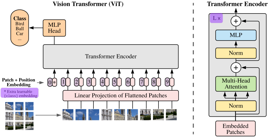
ViT keeps the original Transformer encoder design. Let’s look at how the model works through some simple equations presented in the paper

(1): Input Sequence Construction

\[z_0 = [x_{class}; x_p^1E; x_p^2E; \dots; x_p^N E] + E_{pos}\]

• $x_p^i \quad$: the $i$-th image patch (flattened)
• $E \quad $: the patch-embedding projection matrix
• $E_{pos}$: the positional embedding
• $x_{class}$: the classification token
• $z_0 \quad$: the full input sequence to the Transformer encoder, consisting of:
  • 1 classification token
  • $N$ patch embeddings
  • plus positional encodings

(2), (3): Transformer Encoder Layers

\[z'_\ell = MSA(LN(z_{\ell-1})) + z_{\ell-1}\] \[z_\ell = MLP(LN(z'_\ell)) + z'_\ell\]

This repeats for $L$ layers.

(4): Final Representation

\[y = LN(z_L^0)\]

• $z_L$: the sequence after the final ($L$-th) Transformer block.
• $z_L^0$: the first token (the [CLS] token).
• $y$: the final output, passed through the MLP head for classfication.

In short:

1. The image is turned into a sequence ($z_0$), which includes patch + positional embedding, and extra learnable [class] embedding
2. Processed layer by layer through transformer encoder, finally outputting ($z_\ell$)
3. Then the first token of the $z_\ell$, $z_\ell^0$ (the cls token) is passed through a layer normalization layer outputting $y$
4. Finally $y$ is passed through a 2-layer MLP head(pre-training), or a linear classifier(fine-tuning).

Scale Over Inductive Bias

The paper clearly noted that ViTs have far less image-specific inductive bias than CNNs.

• In CNNs, properties like locality, two-dimensional neighborhood structure, and translation equivariance are baked into every layer. Convolutions naturally capture local pixel patterns and preserve spatial hierarchies.
• In ViTs, the self-attention layers are global by design: every patch can attend to every other patch, regardless of distance.
• The MLP layers are position-wise (applied independently to each token), which makes them translation-equivariant at the token level, but they do not capture local pixel neighborhoods the way convolutions do.
• The 2D structure is used only twice:
  • At the start, by cutting the image into patches.
  • At fine-tuning time, when adjusting positional embeddings for different resolutions.
• Aside from this, the positional embeddings contain no explicit 2D spatial information. This means all spatial relations between patches must be learned from scratch.

This design explains why ViTs underperform CNNs on smaller datasets but excel once scaled to large data and model sizes.

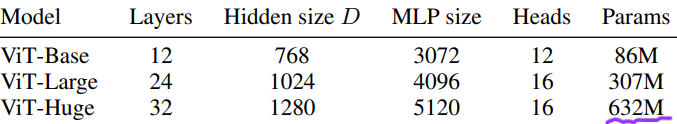
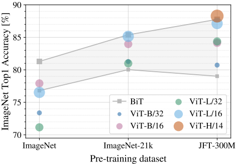
Model Size & Dataset Size

• On small datasets (like ImageNet-1k), ViTs underperform compared to CNNs
• On ImageNet-21k, ViTs and ResNet performed similarly.
• Only after pre-training with the JFT-300M dataset ViTs HUGE model outperformed.

The pros and cons have become very clear at this point.

Since ViTs lack the image-specific inductive bias that CNNs possess, they underperform on small datasets. However, with huge dataset and models that are deep enough (632M parameters), they can outperform current SOTA image classification models; even with its simple and straight forward architecture.

Self-Supervision

One of the key drivers of Transformers’ success in NLP was not just the architecture itself, but large-scale self-supervised pre-training. Models like BERT (Devlin et al., 2019) and GPT (Radford et al., 2018) learned powerful representations by predicting masked words or the next word in a sentence — allowing them to leverage massive amounts of unlabeled text.

The ViT paper explores whether a similar strategy can help in computer vision.

Masked Patch Prediction

To mimic BERT’s masked language modeling, ViT applies masked patch prediction:

• During training, some image patches are masked out (hidden from the model).
• The model is trained to predict the embeddings of the missing patches from the visible ones.
• This encourages the Transformer to learn semantic relationships between patches, much like how BERT learns contextual relationships between words.

*Unlike later approaches such as MAE (He et al., 2022) or BEiT (Bao et al., 2021), the original ViT did not attempt to reconstruct raw pixel values. Instead, it focused on predicting patch embeddings.

Anyways the paper tried the masked patch prediction with the ViT-B/16 model and got:

• 79.9% accuracy on ImageNet, which is about a 2% improvement over training from scratch
• though still around 4% lower than results from supervised pre-training.

Final Thoughts

With deep enough models and big enough data, ViT outperforms previous SOTA models. The paper made it very clear that ViTs lack CNNs’ inductive bias, thus the data-hungry nature of ViTs.

Well then, somebody must have thought of a way to integrate the inductive bias of CNNs into ViTs, right? That’s why I am also going to review CvT: Introducing Convolutions to Vision Transformers.

So…tune in for the next blog post! See you around.

References

1. Bao, H., Dong, L., & Wei, F. (2021). BEiT: BERT Pre-Training of Image Transformers. arXiv preprint arXiv:2106.08254.
   https://arxiv.org/abs/2106.08254
2. Dosovitskiy, A., Beyer, L., Kolesnikov, A., Weissenborn, D., Zhai, X., Unterthiner, T., … & Houlsby, N. (2021). An image is worth 16x16 words: Transformers for image recognition at scale. International Conference on Learning Representations (ICLR).
   https://arxiv.org/abs/2010.11929
3. He, K., Chen, X., Xie, S., Li, Y., Dollár, P., & Girshick, R. (2022). Masked Autoencoders Are Scalable Vision Learners. Proceedings of the IEEE/CVF Conference on Computer Vision and Pattern Recognition (CVPR), 16000–16009. https://arxiv.org/abs/2111.06377

Written by

Roger Kim