Understanding Denoising Diffusion Probabilistic Models
Introduction
As a part of a group study session at my college’s artificial intelligence club HYU HAI, I came across the Denoising Diffusion Probabilistic Models paper. We studied the paper together, and here’s what I learned from it.
Citation
[1] J. Ho, A. Jain, and P. Abbeel, “Denoising Diffusion Probabilistic Models,” arXiv:2006.11239 [cs, stat], Dec. 2020, Available: https://arxiv.org/abs/2006.11239
[2] Kingma, Diederik P., and Max Welling. “Auto-encoding variational bayes.” 20 Dec. 2013, Available: https://arxiv.org/abs/1312.6114
[3] MyeonGu Jo’s GitHub repository Available: https://github.com/MyeongGuJo?tab=repositories
Forward Process
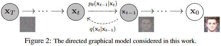
Forward process is the process of adding noise to an image. It is also called diffusion process. Let the original image be represented by $X_0$. The forward process is defined as
\[q(X_{1:T}|X_0) := \prod_{t=1}^{T} q(X_t|X_{t-1})\] \[q(X_t|X_{t-1}) := \mathcal{N}(X_t; \sqrt{1 - \beta_t} X_{t-1}, \beta_t I)\]According to this definition, the calculation needs to be done $T$ times in order to reach the final state, $X_T$, forming a Markov chain. This can be computationally expansive. In order to solve this problem, the paper cites Auto-encoding variational Bayes paper [2], and reparameterizes the diffusion process into
\[q(X_t | X_0) = \mathcal{N}(X_t; \sqrt{\bar{\alpha}_t} X_0, (1 - \bar{\alpha}_t) I)\]where

Notice how the diffusion process is now defined as a single gaussian distribution, with a new parameter $\alpha$. This reparameterization allow us to skip the markov chain and directly reach the image with noise at step $t$, $X_t$.
Now, the paper further reparameterizes them in terms of $\tilde{\mu}_t$ and $\tilde{\beta}_t$. These parameters will later be used for direct comparison between the reverse process’s values in the loss function. Now the forward process takes the final form of
\[q(X_t | X_0) = \mathcal{N}(X_t; \tilde{\mu}_t (X_t, X_0), \tilde{\beta}_t I)\] \[\tilde{\mu}_t(X_t, X_0) := \frac{\sqrt{\bar{\alpha}_t - 1} \beta_t}{1 - \bar{\alpha}_t} X_0 + \frac{\sqrt{\alpha_t (1 - \bar{\alpha}_{t-1})}}{1 - \bar{\alpha}_t} X_t\] \[\quad \tilde{\beta}_t := \frac{1 - \bar{\alpha}_{t-1}}{1 - \bar{\alpha}_t} \beta_t\]These reparametrizations gave me headahces; but here’s how I understand it. ~μt is basically the answer for the diffusion process’s posterior’s expacted value. It is the value that we are aiming to predict using our neural network. ~Bt represents the variability of the noise in the diffusion process, influencing how much the original data gets altered.
Reverse Process
Now, the goal of this paper is to denoise that $X_T$ image back into $X_0$. In order to do that, a reverse process is defined as follow.
\[p_\theta(X_{0:T}) := p(X_T) \prod_{t=1}^{T} p_\theta(X_{t-1}|X_t)\] \[p_\theta(X_{t-1}|X_t) := \mathcal{N}(X_{t-1}; \mu_\theta(X_t, t),\sum_\theta(X_t, t))\]Notice how there is a little $\theta$ under the $p$ function, $\mu$ function and the $\sum$ function? That represents that the value of those functions can be altered by the parameters, which will be calculated by neural network.
Loss Function
Now, in order to train our neural network to get $\tilde{\mu}_t$, we need to define loss function. The loss function used here is defiend based on the variational bound on negative log likelihood.
Given a negative log likelihood $\mathbb{E} [-\log p_\theta(X_0)]$, the paper takes variational bound on that likelihood via the following equation and defines the Loss function $L$
\[\mathbb{E}[-\log p_{\theta}(X_0)]\] \[\leq \mathbb{E}_q[-\log \frac{p_{\theta}(X_{0:T})}{q(X_{1:T}|X_0)}]\] \[= \mathbb{E}_q[-\log p(X_T) - \sum_{t\geq1} \log \frac{p_{\theta}(X_{t-1}|X_t)}{q(X_t|X_{t-1})}] =: L\]To represent the mean $\mu_\theta(X_t, t)$, the paper proposes a specific parameterization motivated by the following analysis of $L_t$. With first setting the variance for the reverse process as $\sigma^2_t I$ we can write:
\[L_{t-1} = \mathbb{E}_{q} \left[ \frac{1}{2 \sigma_{t}^{2}} \| \tilde{\mu}_{t}(x_{t}, x_{0}) - \mu_{0}(x_{t}, t) \|^{2} \right] + C\]Then, we can just simply rewrite it in terms of $\epsilon$, the guassian noise added to the image \(L_{t-1} = \mathbb{E}_{x_0, \epsilon} \left[ \frac{1}{2 \sigma_t^2} \left\| \frac{1}{\sqrt{\alpha_t}} \left( x_t(x_0, \epsilon) - \frac{\beta_t}{\sqrt{1 - \alpha_t}} \epsilon \right) - \mu_0(x_t(x_0, \epsilon), t) \right\|^2 \right]\)
Notice how the expacted value is now represented by $X_0$ and $\epsilon$, $\alpha$ and $\mu_\theta$. The expacted value is also continuosly simplified later in the paper, but I am just going to mention the simple loss function (equation (14)).
\[L_{\text{simple}}(\theta) := \mathbb{E}_{t, x_0, \epsilon} \left[ \left\| \epsilon - \epsilon_\theta \left( \sqrt{\bar{\alpha}_t} x_0 + \sqrt{1 - \bar{\alpha}_t} \epsilon, t \right) \right\|^2 \right]\]Summerizing the mathematical concepts
“To summarize, we can train the reverse process mean function approximator $\mu_\theta$ to predict $\tilde{\mu}_\theta$, or by modifying its parameterization, we can train it to predict $\epsilon$” [1].
That is just basically what we are trying to do, and why the paper reparametrized the functions.
Algorithms
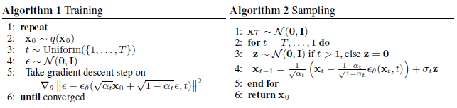

Algorithm 1 is the process of training the neural networking using the loss function defined above (with $\epsilon$). You can see how we take gradient descent step to train our neural network so that the $\hat{\mu_t}$ gets close to $\mu_\theta$.
Algorithm 2 is the process of calculating $X_0$ from $X_T$ using our reverse function and the parameters.
Algorithm 3 and Algorithm 4 is the sender and the receiver for the image. The sender encodes the image using $X_t$ ~ q(X_T|X_0). The receiver decodes the image using revers process function.
The Neural Network
The paper shares the result of its training using neural network. The evaluation using RSME is like the image below. The paper used U-Net backbone neural network. “To represent the reverse process, we use a U-Net backbone similar to an unmasked PixelCNN++” [1].
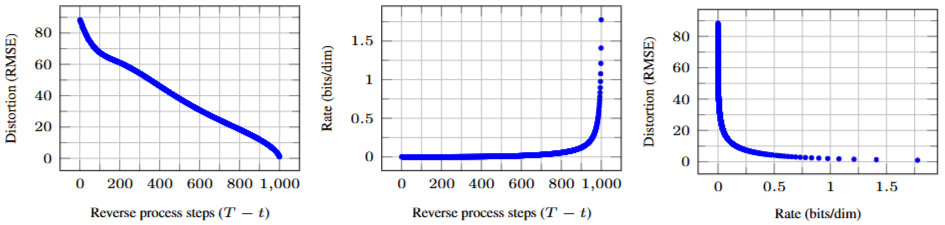 From J. Ho., et al., DDPM, 2020, Figure 5: Unconditional CIFAR10 test set rate-distortion vs. time. Distortion is measured in root mean squared error on a [0, 255] scale. See Table 4 for details.
Code Implementation
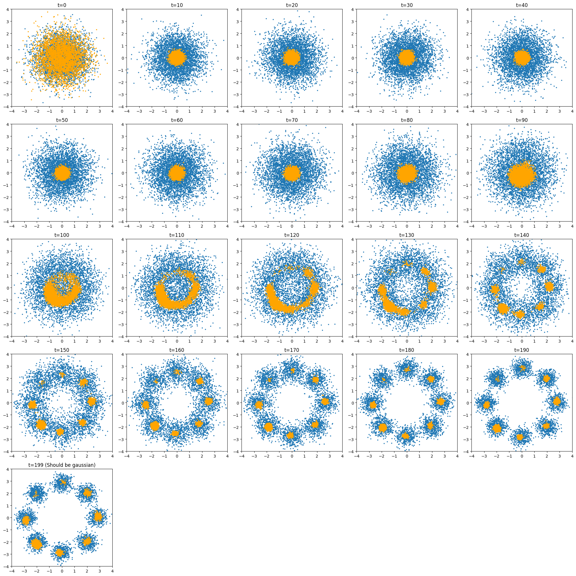 The person who taught me all this, MyeonGu Jo from Hanyang University, has a simple walk-through google colab file that implements this paper. In this specific repository he used Multi-Layer Perceptron for a basic demonstration. You can visit the repository here
Click on the Open in Colab button to run it yourself.
Or checkout his U-Net implementation here
Written by
Roger Kim

